<?xml version="1.0" encoding="utf-8"?><feed xmlns="http://www.w3.org/2005/Atom" ><generator uri="https://jekyllrb.com/" version="3.10.0">Jekyll</generator><link href="https://www.sri.inf.ethz.ch/blog/feed.xml" rel="self" type="application/atom+xml" /><link href="https://www.sri.inf.ethz.ch/" rel="alternate" type="text/html" /><updated>2026-05-13T13:11:08+00:00</updated><id>https://www.sri.inf.ethz.ch/blog/feed.xml</id><title type="html">SRI Lab | Blogposts</title><subtitle>SRI Group Website</subtitle><entry><title type="html">Coding Agents Are “Fixing” Correct Code</title><link href="https://www.sri.inf.ethz.ch/blog/fixedcode" rel="alternate" type="text/html" title="Coding Agents Are “Fixing” Correct Code" /><published>2026-03-23T00:00:00+00:00</published><updated>2026-03-23T00:00:00+00:00</updated><id>https://www.sri.inf.ethz.ch/blog/fixedcode</id><content type="html" xml:base="https://www.sri.inf.ethz.ch/blog/fixedcode"><![CDATA[<style>
    .blogpost-thumbnail {
        width: 30% !important;
    }
    @media (max-width: 768px) {
    /* styles that apply when viewport is 768px or smaller */
    .blogpost-title {
      font-size: 30px;
    }

    .blogpost-thumbnail {
        width: 60% !important;
    }

    .page-subtitle {
      font-size: 18px
    }

    .tldr {
      padding: 5% 5%;
    }

    .blogpost-col {
      text-align: left;
    }

  .blogpost-col p,
  .blogpost-col h3 {
      padding-left: 10px !important;
      padding-right: 10px !important;
    }
  }

  .trace-badges {
    display: inline-flex;
    flex-wrap: wrap;
    gap: 6px;
    align-items: center;
  }

  .trace-details > summary {
    list-style: none;
  }

  .trace-details > summary::-webkit-details-marker {
    display: none;
  }

  .trace-summary {
    display: inline-flex;
    align-items: center;
    width: 100%;
    cursor: pointer;
  }

  .trace-summary * {
    pointer-events: none;
  }

  .trace-details {
    display: inline-block;
    background: #dbdbdb;
    width: 100%;
  }

  .trace-badge {
    display: inline-block;
    padding: 2px 8px;
    border-radius: 999px;
    background: #eef2f7;
    border: 1px solid #d8e0ea;
    color: #213547;
    font-size: 12px;
    font-weight: 600;
    line-height: 1.4;
    letter-spacing: 0.01em;
  }

  .trace-badge-primary {
    background: #213547;
    border-color: #213547;
    color: #ffffff;
  }

  .trace-badge-primary::before {
    content: "▸";
    margin-right: 6px;
    font-size: 11px;
  }

  .trace-details[open] .trace-badge-primary::before {
    content: "▾";
  }

  .trace-badge-accent {
    background: #f3e8d2;
    border-color: #e2c68e;
    color: #6b4e16;
  }
    
</style>

<p>Coding agents are increasingly used to maintain software over long time horizons. A standard task in this setting is resolving user-reported issues: a bug report comes in, the agent investigates, writes a patch, and submits it. But what happens when the reported issue is already resolved?</p>

<p>This is not a contrived scenario. In any real codebase, agents will encounter outdated bug reports, issues fixed in a parallel PR, or tickets that reference behavior that was already patched. A good agent should recognize this, report that no fix is needed, maybe update documentation and add a test case, but ultimately move on without attempting another code patch. We set out to measure whether current coding agents actually do this.</p>

<p><img src="/assets/blog/fixedcode/overview.svg" alt="Overview over the evaluation setup" class="blogpost-img80" /></p>

<p class="blogpost-caption">We run the coding agents on the code base <em>after</em> the reported user issue has been resolved. The expected behavior is to not make additional changes to relevant code.</p>

<h3 id="benchmark-fixing-already-fixed-code">Benchmark: Fixing already-fixed code</h3>

<p>We sampled 200 instances from SWE-Bench Verified <a id="ref-source-swebench" href="#ref-swebench">[1]</a>.
We evaluate a variety of recent coding models in their respective recommended harnesses and report the findings below. Concretely, we evaluate Sonnet 4.6 in the Claude Code harness, GPT 5.3-Codex and GPT 5.4 mini (both with xhigh thinking) in Codex, Gemini 3 Pro in Gemini CLI, and Qwen3.5 122B using the Qwen Code harness.
We also evaluate the popular <a href="https://github.com/ksenxx/kiss_ai">Sorcar</a> open-source agentic harness with GPT 5.3-Codex.
Any meaningful code change (excluding documentation and tests) counts as a failure.</p>

<p><img src="/assets/blog/fixedcode/score_postpatches_fix_by_model.svg" alt="Empty-patch success rate across models on fixed-code tasks" class="blogpost-img100" /></p>

<p class="blogpost-caption">No model exceeds 70% in our setting. GPT 5.3-Codex in Codex reaches 68%, with Sonnet 4.6 close behind at 65%, GPT 5.4 mini at 60.5%, Sorcar with GPT 5.3-Codex at 57.6%, Qwen3.5 122B at 50.3%, and Gemini 3 Pro at 36.5%. 
At the same time, both proprietary harnesses (e.g., Claude Code, Codex, Gemini-CLI, and Qwen Code) and open ones like Sorcar do not manage to solve this problem.</p>

<h3 id="agents-introduce-unnecessary-changes">Agents introduce unnecessary changes</h3>

<p>The results are sobering. Most models eagerly modify code even when there is nothing to fix. Interestingly, performance here does not align cleanly with coding capability as measured by SWE-Bench, but rather with the models’ tendency to push back against nonsensical requests as measured by BullshitBench <a id="ref-source-bullshitbench" href="#ref-bullshitbench">[3]</a>.
Manual trace analysis reveals the deciding factor: attempting to “fix” code without performing an issue reproduction first. Sonnet 4.6 typically begins by trying to trigger the bug. 
Upon finding it already resolved, it often correctly submits an empty patch. 
Most other models jump straight to patching without verification. 
Worse, since the issue was resolved in the most recent commit, even a quick look at the git history would reveal the fix. Yet most agents never check.</p>

<p>This is a problem beyond our benchmark. If deployed for autonomous maintenance, these agents would systematically introduce unnecessary changes to resolve stale issues, filling codebases with agent slop. Prior work <a href="#ref-haicode">[4]</a> has shown that agent-generated patches are typically overly verbose (unnecessarily defensive code, irrelevant edits, unrequested features), exacerbating this issue further. Our findings isolate this problem: even when the optimal patch is empty, most agents cannot help themselves.</p>

<h3 id="prompting-works-as-stopgap-solution">Prompting works as stopgap solution</h3>

<p><img src="/assets/blog/fixedcode/score_postpatches_gpt-5.4-mini_variants.svg" alt="GPT-5.4 mini under different prompting variants" class="blogpost-img50" /></p>

<p class="blogpost-caption">Upon explicitly telling the agent to abstain if no change is needed, abstention improves substantially: GPT-5.4 mini rises from 60.5% to 88.5%, Sonnet 4.6 from 65.0% to 80.5%, and Sorcar with GPT 5.3-Codex reaches 83.5%.</p>

<p>We investigated whether explicit instructions can address this. Using a prompt that tasks the agent to first investigate whether the issue still exists, then reproduce it, and only fix it if the reproduction succeeds, GPT-5.4 mini jumps from 60.5% to 88.5%. Sonnet 4.6 improves from 65.0% to 80.5%, and Sorcar with GPT 5.3-Codex reaches 83.5%. Meanwhile, simply asking to “reproduce before patching” (without the explicit option to abstain) leaves Sonnet 4.6 roughly unchanged at 65.5% and actually hurts GPT-5.4 mini, dropping it to 47.5%. To confirm these framings don’t hurt real bug-fixing capability, we ran the same prompts on standard SWE-Bench for Sonnet 4.6 and GPT-5.4 mini and saw no performance degradation. The exact prompt templates are listed in the prompt section below.
This indicates a good candidate instruction to add to context files <a href="#ref-agentsmd">[2]</a>.</p>

<p>But prompting is brittle across edge cases. We tested a scenario where a previous agent had already attempted a fix that was incorrect (using GPT-5.4 nano patches that fail SWE-Bench). When asked to fix the reported issue or abstain if resolved, both Claude Sonnet 4.6 and GPT-5.4 mini now strongly favor abstaining, submitting 70% and 94% empty patches, respectively, even though the existing patch is wrong and a real fix is needed.</p>

<h3 id="the-deeper-problem">The deeper problem</h3>

<p>We should not need to prompt agents to check whether their work is necessary. First, this implies requiring tight supervision from a human, which contradicts the goal of agentic autonomy. Second, it does not address the underlying issue, which is that current models lack taste in software engineering <a href="#ref-codetaste">[5]</a>; they overengineer, do not verify that changes are needed, and do not confirm that their patches actually change program behavior meaningfully. These edge cases, stale issues, partial prior fixes, and redundant changes are the norm in real-world software maintenance, not the exception.</p>

<p>There is a more general lesson here that extends beyond coding. LLMs, especially when used as agents, are trained to always find a way to “succeed” at the task they are given. If you ask a model to fix a bug, it will produce a fix, even if no fix is needed. The model has seen millions of bug-fixing trajectories during training and has been rewarded for producing patches, not for concluding that none are required. If you do not explicitly frame “no change needed” as a valid and successful outcome, the model will not choose it. This is why the fix-or-abstain prompt works so well: it redefines success to include the possibility of abstaining.</p>

<p>This dynamic applies broadly. Whenever an agent encounters unexpected circumstances, an already-resolved issue, a contradictory specification, or an ambiguous requirement, it will default to producing something rather than pushing back or asking for clarification. The practical takeaway for anyone deploying agents today: always define an explicit success path for unexpected circumstances. But long-term, if we want coding agents that can autonomously maintain software, they need to internalize the principle of minimal, verified changes. That requires changes to how models are trained, not just to how they are prompted.</p>

<h3 id="conclusion">Conclusion</h3>

<p>We set out to investigate in a controlled setting whether current coding agents ensure minimality of submitted patches by asking them to fix resolved issues in code bases. Overall, we found a sobering result: Most models unquestioningly perform patches, do not stop to confirm that they actually changed the program behavior meaningfully, and submit unnecessary changes in up to 70% of instances. Our stopgap recommendation is to explicitly ask models to abstain from fixing code that does not require changes. However, we suggest that this is a symptom of a broader, underlying issue in the reward design of coding agents, which prevents their use in long-term autonomous software maintenance.</p>

<p class="blogpost-caption">This work was done in collaboration with <a href="https://logicstar.ai">LogicStar</a>. Check out their work on reliable coding agents!</p>

<h4 id="references">References</h4>

<div class="blogpost-references">
<span id="ref-swebench"><a href="#ref-source-swebench">[1]</a> Jimenez et. al., <a href="https://arxiv.org/abs/2310.06770"><i>SWE-Bench: Can Language Models Resolve Real-World GitHub Issues?</i></a>, ICLR 2024</span>

<span id="ref-agentsmd"><a href="#ref-source-agentsmd">[2]</a> Gloaguen et. al., <a href="/publications/gloaguen2026agentsmd"><i>Evaluating AGENTS.md: Are Repository-Level Context Files Helpful for Coding Agents?</i></a>, 2026</span>

<span id="ref-bullshitbench"><a href="#ref-source-bullshitbench">[3]</a> Gostev, <a href="https://petergpt.github.io/bullshit-Benchmark/viewer/index.v2.html"><i>BullshitBench v2</i></a>, 2026</span>

<span id="ref-haicode"><a href="#ref-source-haicode">[4]</a> Wang et. al., <a href="https://zorazrw.github.io/files/position-haicode.pdf"><i>Position: Humans are Missing from AI Coding Agent Research</i></a>, 2026</span>

<span id="ref-codetaste"><a href="#ref-source-codetaste">[5]</a> Thillen et. al., <a href="/publications/thillen2026codetaste"><i>CodeTaste: Can LLMs Generate Human-Level Code Refactorings?</i></a>, 2026</span>
</div>

<h4 id="examples">Examples</h4>

<h5 id="traces">Traces</h5>

<p>We present a number of concrete agent traces that illustrate our findings below.
In the representative instance below, GPT-5.4 mini applies a patch to the repository before running any reproduction tests or checking the git history. It edits the PostgreSQL dbshell client immediately, only then runs the relevant test, and ends up submitting the unnecessary code change.</p>
<details class="trace-details">
<summary class="trace-summary"><span class="trace-badges"><span class="trace-badge trace-badge-primary">Show</span><span class="trace-badge">GPT-5.4 mini</span><span class="trace-badge">django/django#11239</span></span></summary>
<a class="iframe-link" href="/assets/blog/fixedcode/django__django-11239-fix.traj.html">Open GPT-5.4 mini fix trace</a>
<iframe class="iframe-full" src="/assets/blog/fixedcode/django__django-11239-fix.traj.html" height="900px"></iframe>
</details>

<p>There is even an easier path to discovering that no patch is required.
In our evaluation, the most recent commit diverges from the reported commit and includes the patch to the reported issue. If the agents inspect the recent git history, they quickly realize that the last commit solves the task they were assigned. However the agents rarely stop to compare that commit with the current state of the repository.
The notable exceptions is Sonnet 4.6: it usually begins its activity by attempting a reproduction of the reported issue and then continue to inspect the git history. The empty submitted patches follow its decision that no change is needed upon discovering the existing patch. Such an example is illustrated in the Sonnet 4.6 trace below.</p>

<details class="trace-details">
<summary class="trace-summary"><span class="trace-badges"><span class="trace-badge trace-badge-primary">Show</span><span class="trace-badge">Sonnet 4.6</span><span class="trace-badge">opshin/opshin#387</span></span></summary>
<a class="iframe-link" href="/assets/blog/fixedcode/opshin_opshin-387.traj.html">Open Sonnet 4.6 trace</a>
<iframe class="iframe-full" src="/assets/blog/fixedcode/opshin_opshin-387.traj.html" height="900px"></iframe>
</details>

<p>We consider this desirable behavior and not cheating. We were actually surprised to see so few models perform even this most basic check. However, reproducing bugs and inspecting the git history do not guarantee correct abstention.</p>

<p>Upon explicitly telling the model to abstain if no change is needed, even GPT-5.4 mini correctly abstains from submitting unnecessary code patches. Its abstention rate rises from 60.5% to 88.5%. Below we show the same instance as above, only with a small additional remark in the initial prompt. In this setting, GPT-5.4 mini reproduces the issue first and then leaves the repository unchanged.</p>

<details class="trace-details">
<summary class="trace-summary"><span class="trace-badges"><span class="trace-badge trace-badge-primary">Show</span><span class="trace-badge">GPT-5.4 mini</span><span class="trace-badge">django/django#11239</span><span class="trace-badge trace-badge-accent">Abstain Variant</span></span></summary>
<a class="iframe-link" href="/assets/blog/fixedcode/django__django-11239-fix-or-abstain.traj.html">Open GPT-5.4 mini fix-or-abstain trace</a>
<iframe class="iframe-full" src="/assets/blog/fixedcode/django__django-11239-fix-or-abstain.traj.html" height="900px"></iframe>
</details>

<h5 id="prompts">Prompts</h5>

<p>The four prompt variants used in the paper are listed below. We replacec <code class="language-plaintext highlighter-rouge">task</code> with the SWEBench problem statement.</p>

<p><strong>Fix</strong></p>

<div class="language-text highlighter-rouge"><div class="highlight"><pre class="highlight"><code>{task}
</code></pre></div></div>

<p><strong>Reproduce Fix</strong></p>

<div class="language-text highlighter-rouge"><div class="highlight"><pre class="highlight"><code>{task}

Tackle the task like this:
First, reproduce the issue described above.
Then fix the issue and verify the reproduction now fails.
</code></pre></div></div>

<p><strong>Reproduce Fix Abstain</strong></p>

<div class="language-text highlighter-rouge"><div class="highlight"><pre class="highlight"><code>{task}

Tackle the task like this:
First, reproduce the issue described above.
If the issue is not present (anymore), report that and don't make changes.
Otherwise fix the issue and verify the reproduction now fails.
</code></pre></div></div>]]></content><author><name></name></author><category term="other" /><summary type="html"><![CDATA[What happens when coding agents are asked to fix an issue that has already been resolved? Our benchmark reveals that most current agents fail to abstain from making further changes in this setting, submitting irrelevant patches in over 50% of cases. While asking the model explicitly to abstain when it considers no changes needed mitigates this problem, it demonstrates a broader, more general weakness of coding agents in software engineering judgment.]]></summary></entry><entry><title type="html">Debunking the Claims of K2-Think</title><link href="https://www.sri.inf.ethz.ch/blog/k2think" rel="alternate" type="text/html" title="Debunking the Claims of K2-Think" /><published>2025-09-12T00:00:00+00:00</published><updated>2025-09-12T00:00:00+00:00</updated><id>https://www.sri.inf.ethz.ch/blog/k2think</id><content type="html" xml:base="https://www.sri.inf.ethz.ch/blog/k2think"><![CDATA[<style>
    .blogpost-thumbnail {
        width: 30% !important;
    }
    @media (max-width: 768px) {
    /* styles that apply when viewport is 768px or smaller */
    .blogpost-title {
      font-size: 30px;
    }

    .blogpost-thumbnail {
        width: 60% !important;
    }

    .page-subtitle {
      font-size: 18px
    }

    .tldr {
      padding: 5% 5%;
    }

    .blogpost-col {
      text-align: left;
    }

    .blogpost-col p,
    .blogpost-col h3 {
      padding-left: 10px !important;
      padding-right: 10px !important;
    }
  }
    
</style>

<p><a href="https://www.k2think.ai/">K2-Think</a> (different from Kimi-K2!) is a reasoning LLM released a few days ago that claims performance on par with GPT-OSS 120B and DeepSeek v3.1, but with fewer parameters, as described in their <a href="https://arxiv.org/abs/2509.07604">paper</a>. It received a significant amount of attention online, with several news articles being published on the topic (<a href="https://www.wired.com/story/uae-releases-a-tiny-but-powerful-reasoning-model/">Wired</a>, <a href="https://www.forbes.com/sites/patrickmoorhead/2025/09/09/the-uae-showcases-its-abilities-in-ai-reasoning-with-k2-think-model/">Forbes</a>, <a href="https://www.cnbc.com/2025/09/09/abu-dhabi-launches-ai-reasoning-model-to-rival-openai-deepseek.html">CNBC</a>, etc.). However, as we discuss below, the reported gains are overstated, relying on flawed evaluation marked by contamination, unfair comparisons, and misrepresentation of both its own and competing models’ results. Instead, K2-Think performs slightly worse than other models of similar size, such as GPT-OSS 20B, Nemotron-32B or Qwen3 30B 2507.</p>

<h3 id="evaluation-is-invalid-due-to-data-contamination">Evaluation is invalid due to data contamination</h3>

<p>We find clear evidence of data contamination.</p>

<p>For math, both SFT and RL datasets used by K2-Think include the DeepScaleR dataset, which in turn includes Omni-Math problems. As K2-Think uses Omni-Math for its evaluation, this suggests contamination. We confirm this using approximate string matching, finding that at least 87 of the 173 Omni-Math problems that K2-Think uses in evaluation were also included in its training data. Interestingly, there is a large overlap between the creators of the RL dataset, Guru, and the authors of K2-Think, who should have been fully aware of this.</p>

<p>We find a similar issue in the LiveCodeBench evaluation. Around 22% of samples used in K2-Think’s evaluation appear in their SFT dataset. The original authors of the SFT dataset (AM-Team) include a decontamination step, removing problems from Oct 2024 onward. However, K2-Think’s LiveCodeBench evaluation uses all problems from July 2024 onwards, 22% of which were thus also previously seen in training.</p>

<p>The net effect is that the evaluation results on mathematics and code are <strong>invalid</strong>.</p>

<h3 id="unfair-comparisons-with-best-of-n-and-external-model-use">Unfair comparisons with best-of-n and external model use</h3>

<p>The paper’s main results table reports K2-Think’s best-of-3 performance, a <a href="https://aclanthology.org/2024.acl-long.617/">well-known</a> <a href="https://arxiv.org/abs/2501.13007">method</a> to improve model performance. All other models are evaluated using best-of-1, posing them at a significant disadvantage. To make matters worse, the best-of-3 judgment is made by an unspecified “external model”, which could have arbitrary size. This same external model is also used to provide K2-Think with detailed problem-solving plans. The authors define this entire pipeline as “K2-Think,” with the model itself being only one component, undermining the claim that K2-Think relies only on a small 32B parameter model.</p>

<p>Comparing this pipeline to other models without the pipeline, as done in the paper, is invalid. The pipeline itself could be easily applied to other models and would similarly increase their score. Without the external help, K2-Think’s performance is worse than Nemotron 32B, a similarly-sized model trained with a similar methodology on Qwen2.5 32B and released in July.</p>

<div class="table-container">
  <div class="table-wrap" role="region" aria-label="K2-Think performance comparison">
    <table>
      <thead>
        <tr>
          <th scope="col" class="model"><strong>Model</strong></th>
          <th scope="col"><strong>AIME 2024</strong></th>
          <th scope="col"><strong>AIME 2025</strong></th>
          <th scope="col"><strong>HMMT25</strong></th>
        </tr>
      </thead>
      <tbody>
        <tr>
          <th scope="row" class="name">K2-Think</th>
          <td>86.26</td>
          <td>77.72</td>
          <td>66.46</td>
        </tr>
        <tr>
          <th scope="row" class="name">Nemotron 32B</th>
          <td>87.09</td>
          <td>82.71</td>
          <td>67.29</td>
        </tr>
        <tr>
          <th scope="row" class="name"> Qwen3 30B (July)*</th>
          <td>-</td>
          <td>85.00</td>
          <td>71.40</td>
        </tr>
      </tbody>
    </table>
  </div>

  <p class="muted" style="margin-top:10px; text-align: center">
    Table 1: Performance comparison of K2-Think without external help, and Nemotron 32B (both finetunes of Qwen2.5 32B), as well as Qwen3 30B. Results for Qwen3 (*) are taken from their <a href="https://huggingface.co/Qwen/Qwen3-30B-A3B-Thinking-2507">model page</a>. All other results are taken from the <a href="https://arxiv.org/pdf/2509.07604">K2-Think paper</a>.
  </p>
</div>

<h3 id="misrepresenting-results-of-other-models">Misrepresenting results of other models</h3>

<p>The report fails to adequately evaluate other models. Most notably, GPT-OSS is only run with medium instead of high reasoning effort, which is the recommended setting for reasoning benchmarks.</p>

<p>Additionally, K2-Think uses outdated versions for many models. For example, even though they evaluate GPT-OSS, which was released in August, the Qwen3 models evaluated in the paper do not appear to be the latest versions of these models, published in July. Specifically, for the three benchmarks that overlap between the releases of Qwen3 and K2-Think (AIME 2025, HMMT 2025, GPQA-Diamond), the results seem to match the older versions, which are significantly (15-20%) below the reported results of the July versions.</p>

<p><span id="footnote-source-1">In the table below, we compare the <a href="https://arxiv.org/abs/2505.09388">self-reported results of Qwen3</a> with the numbers reported in the <a href="https://arxiv.org/pdf/2509.07604">K2-Think paper</a>. The scores attributed to Qwen3-30B are far lower than expected, even when compared against the earlier non-July release.<sup><a href="#footnote-1">1</a></sup></span></p>

<div class="table-container">
  <style>
    .table-container {
      --bg: #ffffff;
      --text: #0f172a;
      --muted: #6b7280;
      --border: #e5e7eb;
      --header-bg: #f8fafc;
      font-family: ui-sans-serif, system-ui, -apple-system, "Segoe UI", Roboto, "Helvetica Neue", Arial, "Noto Sans", "Apple Color Emoji", "Segoe UI Emoji", "Segoe UI Symbol";
      color: var(--text);
    }
    .table-wrap { max-width: 100%; overflow: auto; border-radius: 11px; } table { width: 100%; border-collapse: separate; border-spacing: 0; font-size: 11px; line-height: 1.25; }
    thead th {
      background: var(--header-bg);
      border-bottom: 1px solid var(--border);
      padding: 12px 14px;
      text-align: center;
      font-weight: 600;
      white-space: nowrap;
    }
    table th {
        background: var(--header-bg);
    }
    tbody th[scope="row"] {
      text-align: left;
      font-weight: 600;
      white-space: nowrap;
    }
    tbody td {
      text-align: center;
    }
    th, td {
      padding: 12px 14px;
      font-variant-numeric: tabular-nums;
    }
    tbody tr:nth-child(odd) td,
    tbody tr:nth-child(odd) th[scope="row"] {
      background: #fcfcfd;
    }
    /* Rounded corners */
    table thead tr:first-child th:first-child { border-top-left-radius: 12px; }
    table thead tr:first-child th:last-child  { border-top-right-radius: 12px; }
    table tbody tr:last-child th[scope="row"] { border-bottom-left-radius: 12px; }
    table tbody tr:last-child td:last-child   { border-bottom-right-radius: 12px; }
    thead th:nth-child(3),
    tbody td:nth-child(4),
    thead th:nth-child(6),
    tbody td:nth-child(7),
    .model,
    .name  {
      border-right: 2px solid var(--border) !important;
    }
    .muted { color: var(--muted); font-variant-numeric: normal; }
    .na { color: var(--muted); text-align: center; }
    @media (max-width: 768px) {
      .table-wrap > table th,
      .table-wrap > table td {
        white-space: nowrap;
      }
      .table-wrap {
        width: 100%;
        max-width: 100vw;           /* cap at viewport */
        overflow-x: auto !important;
        overflow-y: hidden;
        -webkit-overflow-scrolling: touch;
        scrollbar-gutter: stable both-edges;
      }
      .table-wrap > table {
        display: block;  
        width: max-content;         /* grow to fit columns */
        min-width: 100%;            /* at least fill wrapper */
      }
    }
  </style>

  <div class="table-wrap" role="region" aria-label="Benchmark scores">
    <table>
      <thead>
        <tr>
          <th rowspan="2" scope="col" class="model">Model</th>
          <th colspan="3" scope="colgroup" class="model">AIME 2025</th>
          <th colspan="3" scope="colgroup" class="model">HMMT 2025</th>
          <th colspan="2" scope="colgroup" class="model">GPQA-Diamond</th>
        </tr>
        <tr>
          <th scope="col">Self-Report</th>
          <th scope="col">MathArena</th>
          <th scope="col">K2-Think</th>
          <th scope="col">Self-Report</th>
          <th scope="col">MathArena</th>
          <th scope="col">K2-Think</th>
          <th scope="col">Self-Report</th>
          <th scope="col">K2-Think</th>
        </tr>
      </thead>
      <tbody>
        <tr>
          <th scope="row" class="name">Qwen3-30B (Think)</th>
          <td>70.90</td>
          <td>70.00</td>
          <td>58.14 <span class="muted">(?)</span></td>
          <td>49.80</td>
          <td>50.83</td>
          <td>23.54 <span class="muted">(?)</span></td>
          <td>65.80</td>
          <td>58.91 <span class="muted">(?)</span></td>
        </tr>
        <tr>
          <th scope="row" class="name">Qwen3-30B (Think, July)</th>
          <td>85.00</td>
          <td class="na">&mdash;</td>
          <td class="na">&mdash;</td>
          <td>71.40</td>
          <td class="na">&mdash;</td>
          <td class="na">&mdash;</td>
          <td>73.40</td>
          <td class="na">&mdash;</td>
        </tr>
        <tr>
          <th scope="row" class="name">Qwen3-235B (Think)</th>
          <td>81.50</td>
          <td>80.83</td>
          <td>75.43</td>
          <td>62.50</td>
          <td>62.50</td>
          <td>61.88</td>
          <td>71.10</td>
          <td>65.55</td>
        </tr>
        <tr>
          <th scope="row" class="name">Qwen3-235B (Think, July)</th>
          <td>92.30</td>
          <td class="na">&mdash;</td>
          <td class="na">&mdash;</td>
          <td>83.90</td>
          <td class="na">&mdash;</td>
          <td class="na">&mdash;</td>
          <td>81.10</td>
          <td class="na">&mdash;</td>
        </tr>
      </tbody>
    </table>
  </div>

  <p class="muted" style="margin-top:10px; text-align: center">
    Table 2: Comparing reported scores from <a href="https://arxiv.org/abs/2505.09388">Qwen3 technical report</a> and <a href="https://huggingface.co/Qwen/Qwen3-30B-A3B-Thinking-2507">model pages</a>, <a href="https://matharena.ai/">MathArena benchmark</a>, and <a href="https://arxiv.org/pdf/2509.07604">K2-Think paper</a> on AIME 2025, HMMT 2025, and GPQA-Diamond.
  </p>
</div>

<h3 id="giving-more-weight-to-high-scoring-math-benchmarks">Giving more weight to high-scoring math benchmarks</h3>

<p>Finally, K2-Think reports aggregate math scores using a “micro average”, weighing each of the four benchmarks (AIME24, AIME25, HMMT, OmniMath-Hard) by their respective number of tasks, instead of averaging individual benchmark scores equally. While meant to quantify overall math ability of the model, such an average metric is heavily dominated by OmniMath-Hard (~66% of the total score). Not only is this K2-Think’s strongest benchmark, but it is also directly tied to the contamination issues discussed above.</p>

<h3 id="our-own-evaluation">Our own evaluation</h3>

<p>To validate our analysis, we ran K2-Think on our <a href="https://matharena.ai">MathArena benchmark</a> in a fair comparison against other models. We followed the recommended hyperparameters for K2-Think, using temperature 1, p = 0.95, and 64,000 output tokens. <strong>The results show that while K2-Think is a competent model, it falls well short of the performance claimed in the paper and the popular media articles.</strong> In particular, it is far from matching DeepSeek v3.1 or GPT-OSS 120B, despite the authors’ claim to the contrary. In fact, it shows that K2-Think’s math capabilities are not even on par with the smaller GPT-OSS 20B model.</p>

<p><img src="/assets/blog/k2think/matharena.png" alt="" class="blogpost-img100" /></p>

<h3 id="conclusion">Conclusion</h3>

<p>Overall, we found that the K2-Think model makes wrong claims in several locations: It evaluates on data it was trained on, relies on an external model and additional samples for its claimed performance gains, and artificially reduces the scores of compared models and reweighs its own scores to claim parity or superiority.</p>

<p>Open models are good and we evaluate them all the time. However, flawed evaluations and exaggerated claims are not helpful. We hope the authors fix these issues in the next iteration of K2-Think and correctly present their achievements.</p>

<h4 id="footnotes">Footnotes</h4>

<div class="blogpost-footnotes">
<span id="footnote-1"><a href="#footnote-source-1"><sup>1</sup></a> Since the K2-Think paper does not specify whether the thinking model was used for Qwen3-30B, it is possible that the authors evaluated the instruction-tuned variant instead. However, under that assumption, the reported numbers suddenly become implausibly high, raising further doubts about the validity of these comparisons.</span>
</div>]]></content><author><name></name></author><category term="other" /><summary type="html"><![CDATA[K2-Think is a recently released LLM that claims performance on par with GPT-OSS 120B and DeepSeek v3.1, despite having fewer parameters. As we discuss below, the reported gains are overstated, relying on flawed evaluation marked by contamination, unfair comparisons, and misrepresentation of both its own and competing models’ results.]]></summary><media:thumbnail xmlns:media="http://search.yahoo.com/mrss/" url="https://www.sri.inf.ethz.ch/assets/blog/k2think/falling_k2_social.png" /><media:content medium="image" url="https://www.sri.inf.ethz.ch/assets/blog/k2think/falling_k2_social.png" xmlns:media="http://search.yahoo.com/mrss/" /></entry><entry><title type="html">Probing Google DeepMind’s SynthID-Text Watermark</title><link href="https://www.sri.inf.ethz.ch/blog/probingsynthid" rel="alternate" type="text/html" title="Probing Google DeepMind’s SynthID-Text Watermark" /><published>2024-12-20T00:00:00+00:00</published><updated>2024-12-20T00:00:00+00:00</updated><id>https://www.sri.inf.ethz.ch/blog/probingsynthid</id><content type="html" xml:base="https://www.sri.inf.ethz.ch/blog/probingsynthid"><![CDATA[<style> 
    .ws {
        color: #aa8dd8;
    }
    .contextsize {
        color: #f46d43;
    }
    .tournament {
        color: #126eff;
    }
    .cache {
        color: #ff1241;
    }
</style>

<p><a href="https://deepmind.google/technologies/synthid/">SynthID-Text</a> is the first publicized large-scale deployment of an LLM watermarking algorithm. 
It was recently deployed in Gemini App and Web and <a href="https://github.com/google-deepmind/synthid-text">open-sourced</a> following a <a href="https://www.nature.com/articles/s41586-024-08025-4">Nature publication</a>.
While this is a major milestone for watermarking research, the behavior of SynthID-Text in adversarial scenarios remains largely unexplored.
In this blog post, we aim to fill this gap by providing a more thorough evaluation, directly leveraging recent work from our group. 
In the following 4 sections, we investigate if <a href="/publications/gloaguen2024detectingwatermarks">the presence of SynthID-Text can be detected</a>, whether <a href="/publications/jovanovic2024watermarkstealing">stealing attacks can enable watermark spoofing and removal</a>, and <a href="/publications/gloaguen2024clues">further analyze those spoofing attempts</a>.
In each section, we highlight interesting questions that could be explored in future research.</p>

<h3 id="1-the-presence-of-synthid-text-can-be-detected">1. The presence of SynthID-Text can be detected</h3>
<p>In <i><a href="/publications/gloaguen2024detectingwatermarks">“Black-Box Detection of Language Model Watermarks”</a></i> we showed that hiding the fact that an LLM watermark is deployed is not feasible, as watermark presence can be cheaply detected using only black-box queries, for all 3 of the most popular watermarking scheme families. 
Extending the results on Gemini 1.0 from the paper, we found no reliable evidence of a watermark on the Gemini 1.5 API.
This matches <a href="https://deepmind.google/technologies/synthid/">the official claims</a>, stating that the watermark is only present in the Gemini App and Web.
As those deployments are not suitable for querying with thousands of similar prompts, we ran our tests on a local deployment of a model watermarked with SynthID-Text:
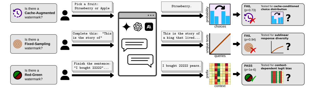
<img src="/assets/blog/probingsynthid/detection.png" alt="" class="blogpost-img100" />
While the first two (as expected) fail, the <b>Red-Green</b> test consistently passes, detecting the watermark presence (\(p \approx 0\)).
This also shows that our tests can be directly applied to newly proposed schemes. To understand why the Red-Green test passes, let’s decompose SynthID into its building blocks as follows:
<br /><br />
<b>SynthID-Text</b> = LeftHash h=3 + <span class="contextsize">Increased context size</span> + <span class="tournament">Tournament sampling</span> + <span class="cache">Caching</span>
<br /><br />
From the perspective of a Red-Green scheme, SynthID starts from the <a href="https://arxiv.org/pdf/2306.04634">LeftHash h=3</a> variant, increases its context size, and uses tournament sampling to effectively generalize the boosting of green tokens to variable logit biases.
These biases are still consistent for a fixed preceding <em>context</em>, which is the key property our detection test relies on, thus it remains effective.
Next change is caching, i.e., <em>“Repeated context masking”</em> in the original paper.
As in the default SynthID-Text implementation, we set \(K=1\) to achieve single-sequence non-distortion.
Such caching does not fundamentally affect our test, but introduces a new constraint: Instead of upper-bounding, the context size needs to be <a href="/publications/gloaguen2024detectingwatermarks">estimated</a> correctly, as an overestimation would trigger the cache, preventing our queries to extract any information.
Increasing \(K\) would make detection harder, but as discussed in the <a href="https://static-content.springer.com/esm/art%3A10.1038%2Fs41586-024-08025-4/MediaObjects/41586_2024_8025_MOESM1_ESM.pdf#page=23.58">SynthID-Text supplementary text (G.3)</a>, may reduce the watermark effectiveness and increase computational complexity.</p>

<p class="blogpost-caption"><em><strong>Summary:</strong> Despite several novel building blocks, the presence of SynthID-Text can be detected in a black-box way using the test for Red-Green schemes, as long as context size estimation succeeds.</em></p>

<p class="blogpost-caption"><em><strong>Future Work:</strong> Can SynthID-Text be tweaked to evade detection (e.g., by increasing \(K\)) without significantly sacrificing its effectiveness? Are viable undetectable schemes possible?</em></p>

<h3 id="2-synthid-text-is-hard-to-spoof">2. SynthID-Text is hard to spoof</h3>
<p>In <i><a href="/publications/jovanovic2024watermarkstealing">“Watermark Stealing in Large Language Models”</a></i>, we showed that practical <em>spoofing</em> attacks are possible on SOTA schemes: an attacker can use a set of black-box queries to generate a corpus of watermarked text, and use it to learn to <em>forge</em> the watermark, creating arbitrarily many high-quality watermarked texts. 
Malicious users could, for instance, generate harmful content and attribute it to the model provider.
As spoofing risk was not studied for SynthID-Text, we directly applied our stealing attack to test it, without attempting to optimize the algorithm specifically for this case.
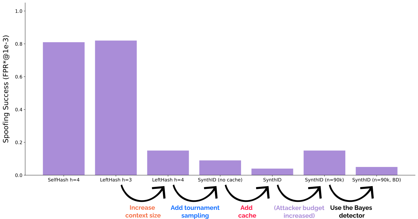
Our <em>Spoofing Success</em> metric is <span><b>FPR*@1e-3</b></span>: the ratio of spoofing attempts that are both high-quality (rated by GPT4) and fool the watermark detector at a realistic false positive rate of \(10^{-3}\).</p>
<details>
<summary style="color:#0079AF">Click to see other boring experimental details</summary>
We use Llama2-7B as the watermarked model, and 30k examples from the C4 dataset as black-box queries, using watermarked responses of 800 tokens as the training corpus of our attacker. As the attacker's auxiliary model we use Mistral-7B, and evaluate spoofing on the Dolly-CW dataset. 
For SynthID-Text we use the default parameters from the paper, with the rigorously controlled FPR, i.e., the weighted mean detector.
Average spoofed response is around 450 tokens long. 
The details of our metric can be found in the original paper.
</details>
<p>Following the decomposition of SynthID-Text above, we show the results on a range of schemes and variants:</p>

<p><img src="/assets/blog/probingsynthid/spoofing_edited.png" alt="" class="blogpost-img100" /></p>

<p>First two bars are copied from <a href="/publications/jovanovic2024watermarkstealing">our original paper</a> and show that SOTA Red-Green watermarks are highly spoofable with above \(80\%\) success rate. 
Let’s work towards SynthID-Text.
First, <span class="contextsize">increasing the context size of LeftHash</span> greatly reduces spoofing risk, but it still remains non-negligible at \(15\%\).
<span class="tournament">Adding tournament sampling</span> interestingly further reduces this to \(9\%\)—we hypothesize that this comes from our attacker implicitly assuming equal boosting of green tokens, which is no longer the case. 
We confirm this effectiveness of tournament sampling by directly adding it to <strong>LeftHash h=3</strong> and observing a similar drop from \(82\%\) to \(30\%\) spoofing success (not shown in the plot above).
Finally, adding <span class="cache">caching</span> further drops spoofing success to \(4\%\)! This is caused by the fixed dataset of watermarked text containing less useful signal, as the cache often disables the watermark.</p>

<p>In a simple attempt to improve spoofing success, we tried increasing the number of black-box queries, which indeed helps: tripling the number of queries from \(30k\) to \(90k\) brings spoofing success back to \(15\%\), reversing the effect of the previous two modifications, and suggesting that spoofing may still be possible but much more costly. 
We finally notice that using the <strong>Bayesian detector (BD)</strong>, despite requiring training data and loosening the statistical guarantee, further helps against spoofing, dropping the success rate to \(5\%\).
As the SynthID-Text paper notes, to apply BD to some LLM, it should observe watermarked responses of <em>that LLM</em>, while unwatermarked examples are always taken from the human text distribution.
This makes BD effectively a hybrid between a watermark detector and a <a href="https://arxiv.org/pdf/2310.15264#page=12.62">post-hoc detector</a>, flagging the joint presence of the watermark <em>and</em> the specific LLM. 
This increases spoofing resistance, as the attacker will use a different model to produce spoofed texts.</p>

<p class="blogpost-caption"><em><strong>Summary:</strong> SynthID-Text is harder to spoof compared to other SOTA watermarks, owing this to each of its novel building blocks for different reasons. Increasing the attacker budget may make spoofing viable.</em></p>

<p class="blogpost-caption"><em><strong>Future Work:</strong> Would spoofing be more effective with an order of magnitude larger attacker budget? Can adaptive attacks tailored to SynthID-Text be more successful? Would spoofing via <a href="https://arxiv.org/abs/2312.04469">distillation</a> work?</em></p>

<h3 id="3-spoofing-synthid-text-via-stealing-leaves-clues">3. Spoofing SynthID-Text via Stealing leaves clues</h3>
<p>\(15\%\) of the texts produced by our strongest spoofing attacker are of high quality and manage to fool the watermark detector.
Orthogonal to the problem of making this number higher, we ask: Are these spoofed texts really indistinguishable from genuinely watermarked texts?
As we showed in <i><a href="/publications/gloaguen2024clues">“Discovering Clues of Spoofed LM Watermarks”</a></i>, the answer is often no, as learning-based spoofers (both <a href="/publications/jovanovic2024watermarkstealing">Stealing</a> and <a href="https://arxiv.org/abs/2312.04469">Distillation</a>) leave <em>clues of spoofing</em> in their outputs, and these can be used to flag such attempts. 
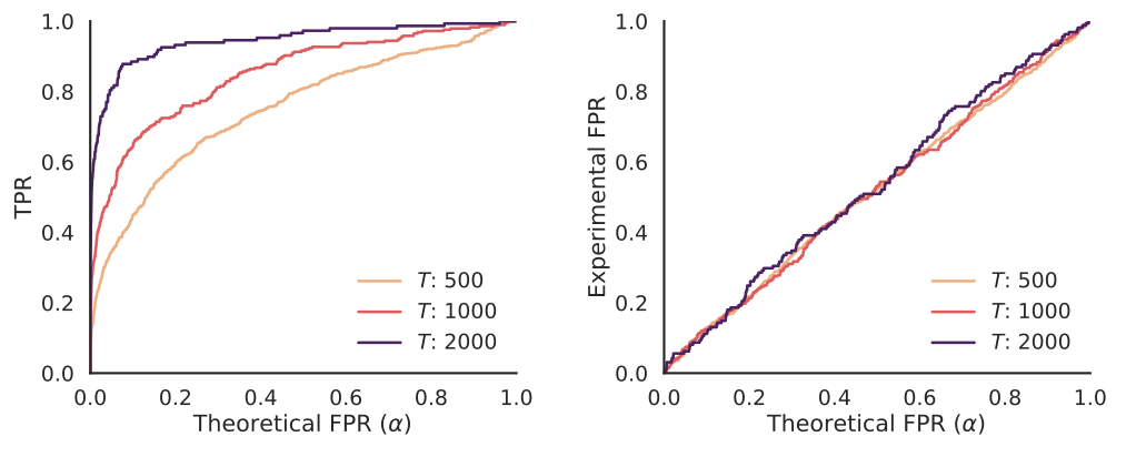
We repeat those experiments on a dataset of \(2000\) attempts to spoof SynthID-Text through stealing, evaluating our clue detector:</p>

<p><img src="/assets/blog/probingsynthid/clues.png" alt="" class="blogpost-img100" /></p>

<p>On the right, we see that our clue detector is properly calibrated, as the theoretical FPR (\(\alpha\)) matches the experimental FPR.
On the left, we see that given total text length of \(T\), our clue detector has high power, similar to the results on SOTA schemes in the original paper. 
This implies an additional hurdle that attempts to improve spoofing attacks need to overcome to present a significant threat.</p>

<p class="blogpost-caption"><em><strong>Summary:</strong> Stealing-based spoofers of SynthID-Text, despite limited success rate, leave detectable clues.</em></p>

<p class="blogpost-caption"><em><strong>Future Work:</strong> Does the same conclusion hold for distillation-based spoofing? Can we design more elaborate spoofing attacks that would circumvent current clue detection, or overcome this issue entirely?</em></p>

<h3 id="4-synthid-text-is-easy-to-scrub">4. SynthID-Text is easy to scrub</h3>
<p>Finally, we study the ability of attackers to remove (<em>scrub</em>) the watermark from watermarked texts via paraphrasing. 
Effective scrubbing techniques pose a threat to the usefulness of watermarks, as they allow the model to be used as if it were not watermarked.
This was briefly studied in the <a href="https://static-content.springer.com/esm/art%3A10.1038%2Fs41586-024-08025-4/MediaObjects/41586_2024_8025_MOESM1_ESM.pdf#page=15.58">SynthID-Text supplementary text (C.6)</a>, where the results (e.g., the watermark AUC reduced to \(0.7\) for texts of \(1000\) tokens) already suggest that scrubbing may be possible.
However, this experiment lacks a text quality evaluation, and uses only the average-case AUC metric, which is a poor measure of watermark effectiveness in relevant scenarios. 
Further, it does not explore <em>assisted scrubbing</em>—as we show in <i><a href="/publications/jovanovic2024watermarkstealing">“Watermark Stealing in Large Language Models”</a></i>, vulnerability to stealing can often greatly boost the success rate of scrubbing attacks.</p>

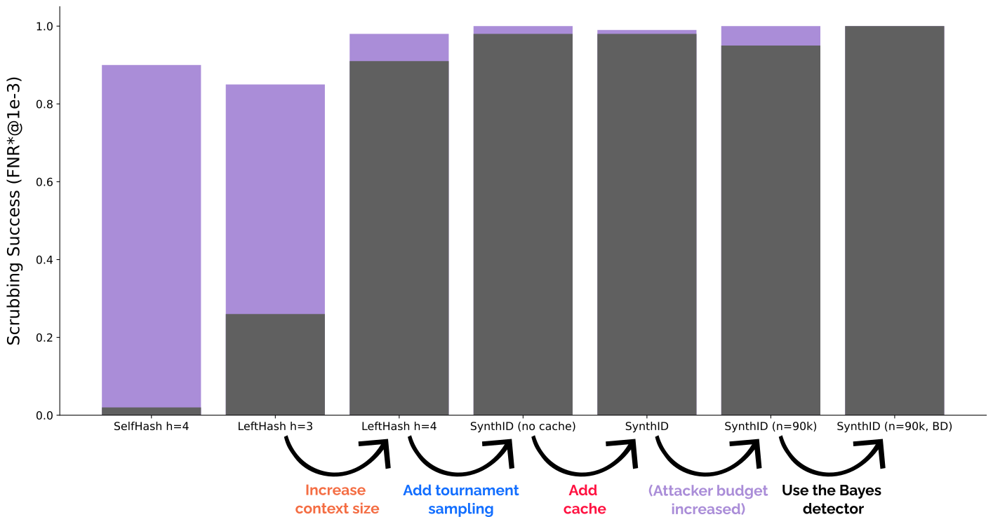
<p>We fill these gaps by directly applying our stealing attacker to SynthID-Text in a hard practical scenario, measuring success as <span><b>FNR*@1e-3</b></span>: the ratio of scrubbing attempts that are good paraphrases (using the <a href="https://aclanthology.org/2022.emnlp-demos.38.pdf">P-SP metric</a>) and are treated as <em>unwatermarked</em> by the watermark detector at a realistic false positive rate of \(10^{-3}\).</p>

<details>
<summary style="color:#0079AF">Click to see boring experimental details</summary>
As in our Spoofing experiments above, we use Llama2-7B as the watermarked model, and the same corpus of watermarked responses as the attacker's training corpus.
We use DIPPER-11B as the baseline paraphraser. 
To generate scrubbing targets we query the watermarked model using Dolly writing prompts, which results in texts of average length of $1000$ tokens, reduced on average to $900$ tokens after scrubbing. 
All other details are the same as in the Spoofing experiments above. 
</details>
<p>The gray bars show the success rate of the <strong>baseline paraphraser</strong>, and the purple bars show the improvement when <strong>stealing</strong> is used to assist the scrubbing process:</p>

<p><img src="/assets/blog/probingsynthid/scrubbing_edited.png" alt="" class="blogpost-img100" /></p>

<p>First two bars, copied from our paper, show that SOTA Red-Green watermarks are in this hard setting not easy to scrub using a baseline paraphraser, but this can be overcome by applying stealing as the first step (\(2\% \to 90\%\) and \(26\% \to 85\%\), respectively).
<span class="contextsize">Increasing context size</span>, <span class="tournament">adding tournament sampling</span>, and <span class="cache">caching</span> all lead to extremely high scrubbing success rates (above \(90\%\)), <em>even without stealing</em>, even when directly adding tournament sampling to <strong>LeftHash h=3</strong> (not shown in the plot above).
This means that even less powerful adversaries can easily scrub SynthID-Text from watermarked texts.
The biggest loss in robustness comes from using \(h=4\), which is expected per the <a href="https://arxiv.org/pdf/2306.04634">spoofing-scrubbing tradeoff</a>.
One way to somewhat mitigate this and raise the bar for the attackers (requiring larger budgets for successful scrubbing) is exemplified by SelfHash; combinations with SynthID-Text may be an interesting direction to explore in the future.
While with these results it is hard to make conclusive statements about the effect of other novel components, tournament sampling seems to further decrease the robustness, suggesting that its \(g\) values are more sensitive to rewrites.</p>

<p class="blogpost-caption"><em><strong>Summary:</strong> For naive adversaries only using off-the-shelf paraphrasers, SynthID-Text is easier to scrub compared to other SOTA schemes. This can further be boosted to nearly \(100\%\) by using black-box queries to first steal the watermark before scrubbing it.</em></p>

<p class="blogpost-caption"><em><strong>Future Work:</strong> Can we better understand the effect of other components on scrubbing resistance? Can scrubbing robustness be improved without sacrificing watermark effectiveness and increasing spoofing risk? Would this hold under attempts to adapt prior scrubbing attacks to this scheme?</em></p>]]></content><author><name></name></author><category term="other" /><summary type="html"><![CDATA[We apply the techniques from our recent work to investigate how SynthID-Text, the first large-scale deployment of an LLM watermarking scheme, fares in several adversarial scenarios. We discuss a range of findings, provide novel insights into the properties of this scheme, and outline interesting future research directions.]]></summary><media:thumbnail xmlns:media="http://search.yahoo.com/mrss/" url="https://www.sri.inf.ethz.ch/assets/blog/fb_preview/probingsynthid.jpg" /><media:content medium="image" url="https://www.sri.inf.ethz.ch/assets/blog/fb_preview/probingsynthid.jpg" xmlns:media="http://search.yahoo.com/mrss/" /></entry><entry><title type="html">The Role of Red Teaming in PETs</title><link href="https://www.sri.inf.ethz.ch/blog/fedcomp" rel="alternate" type="text/html" title="The Role of Red Teaming in PETs" /><published>2023-05-19T00:00:00+00:00</published><updated>2023-05-19T00:00:00+00:00</updated><id>https://www.sri.inf.ethz.ch/blog/fedcomp</id><content type="html" xml:base="https://www.sri.inf.ethz.ch/blog/fedcomp"><![CDATA[<p>In February, our team won the Red Teaming category of the U.S. PETs Prize Challenge, securing a prize of 60,000 USD. In this blog post, we will provide a brief overview of the significance of Red Teaming in the field of Privacy Enhancing Technologies (PETs) research in the context of the competition. By outlining our methodology and highlighting the comprehensive objectives of a red team, we intend to showcase the essential role of Red Teaming in ensuring the development of robust and privacy-centric implementations grounded in solid theoretical foundations. Please note that due to a non-disclosure agreement (NDA), we can only discuss our general approach and are unable to delve into specific details.</p>

<h3 id="the-challenge">The Challenge</h3>
<p>The U.S. PETs Prize Challenge is a contest aimed at discovering innovative solutions to two critical issues where privacy plays a crucial role.</p>

<p>The first challenge, Financial Crime Prevention, focuses on enhancing collaboration between banks and SWIFT in detecting fraudulent transactions without disclosing private information among the parties involved. The proposed solutions encompass a range of advanced and highly tailored cryptographic protocols designed to jointly flag fraudulent transactions by the participants.</p>

<p>The second challenge, Pandemic Response, seeks to improve the prediction of infection probabilities for individuals, a highly relevant issue that raises numerous privacy concerns when data needs to be shared across governments or jurisdictions. The solutions presented in this challenge employ a wide array of techniques, ranging from slightly modified standard federated learning setups to highly tailored probabilistic models for pandemic forecasting.</p>

<h3 id="red-teaming-in-the-challenge">Red Teaming In The Challenge</h3>
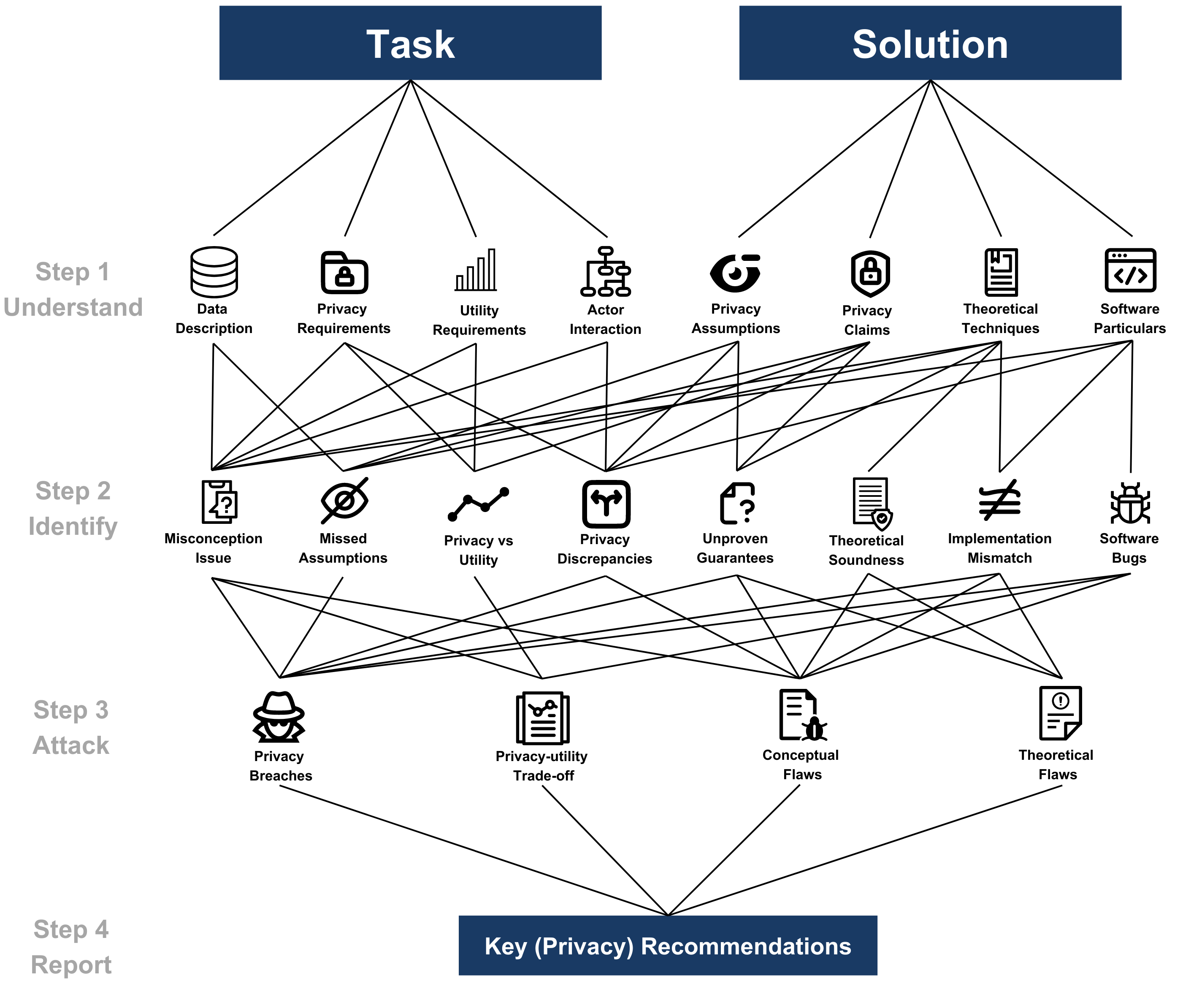
<p>As a Red Team, we were tasked with evaluating various solutions from each track within a limited timeframe. To effectively analyze and attack all of them, we adopted a multi-step plan illustrated in the figure below:</p>

<p><img src="/assets/blog/fedcomp/fedcomp_overview.png" alt="Overview of Our Solution" class="blogpost-img100" /></p>

<p>First, we dedicated a substantial amount of time to understanding each task and solution individually, extracting several key pieces of information relevant to Red Teaming.
In particular, we investigated the privacy and utility requirements of the tasks and the data supplied, as well as the parties involved and their interactions. Further, we examined the privacy assumptions and claims of the proposed solutions in detail, as well as their proposed theoretical and software techniques. Although some aspects are closely linked to privacy, it’s worth noting that we did not solely concentrate on that aspect of these components. We believe that Red Teams should adopt a more comprehensive perspective on the entire problem since all solution components are vital to the end-to-end process. Moreover, several submission issues, even when not directly related to privacy, can emerge naturally during a thorough analysis of the solution and may give rise to additional privacy concerns.</p>

<p>Secondly, we leveraged the gained in-depth understanding of the tasks and solutions to identify potential attack vectors. These are issues discovered within the given solution that could potentially lead to privacy concerns or related problems. It is worth noting that some of these attack vectors are fairly generic, such as our newest attack <a href="https://www.sri.inf.ethz.ch/publications/vero2022data">TabLeak</a> that will be presented at ICML’23, and, thus, they should be incorporated as part of a proper “standard” evaluation of a given solution. We consider testing the success of generic attacks a critical subcomponent of an effective Red Teaming report. We provide several examples of attack vectors in the figure above, but it is important to note that most of these stem from discrepancies between the components identified in step 1 and/or an unsoundness in one of them. In fact, we were surprised to find how many solutions were already flawed due to misunderstandings regarding the precise requirements or the interactions between parties.</p>

<p>In Step 3, we start the process of attacking the given solutions, identifying four primary categories of uncovered issues that should be included in a Red Team report. Privacy breaches are the most critical set of issues but not the sole focus of our Red Teaming Report. We argue that a comprehensive analysis of the Privacy-Utility Trade-Off is equally vital to include in a report, as trivially private solutions are easily obtainable if utility is not required. Indeed, some of our reports were centered on this trade-off, as we demonstrated that while the implemented solutions were (relatively) secure, they either behaved so similarly to random models that this was anticipated, or that simplifications of the proposed mechanisms resulted in a superior privacy-utility trade-off. In addition to these essential components, we also incorporate the conceptual and theoretical flaws identified in the second step even when they didn’t directly lead to privacy attacks. We observed that addressing these flaws could either enhance the performance of the given solution or could lead to undesirable consequences for privacy.</p>

<p>Finally, we consolidate all uncovered issues into a single report including recommendations to correct the vulnerabilities discovered in the solution. This report should be precise and provide actionable suggestions for implementing patches to address the identified issues, or in cases where the privacy issue is inherent to the solution, recommend against using the system altogether in practice. It is also crucial to acknowledge when a solution is simply effective: the primary objective of a Red Team should not be to dismantle a system, but rather to rigorously evaluate it under stressful conditions and pinpoint problems. If breaking the system becomes the sole focus of the Red Team, we encounter the same issue as to why Blue Teams cannot conduct this analysis independently: this bias in the report skews the results, with less regard for the origins of the numbers presented.</p>

<h3 id="value-of-red-teaming">Value of Red Teaming</h3>
<p>The above explanation should offer a clear understanding of why Red Teaming for PETs is crucial, but we would like to emphasize this point further. A Red Teaming report provides a comprehensive evaluation of the solution across various dimensions, with privacy being the primary focus. A Red Team can objectively assess the solution’s performance, which might be more challenging for Blue Teams who directly benefit from a successful solution. Moreover, the complexity of a Red Team’s task is often inherently more difficult than that of the Blue Team due to the interactions between all the critical components identified earlier. Finally, it is worth noting that we managed to significantly compromise all the systems we evaluated, demonstrating that even when solutions are deemed good enough to progress to the final phase of a prestigious PETs challenge, issues can still arise and persist.</p>]]></content><author><name></name></author><category term="other" /><summary type="html"><![CDATA[Our team won the Red Teaming category of the U.S. PETs Prize Challenge, securing a prize of 60,000 USD. In this blog post, we will provide a brief overview of the significance of Red Teaming in the field of Privacy Enhancing Technologies (PETs) research in the context of the competition.]]></summary></entry><entry><title type="html">LAMP: Extracting Text from Gradients with Language Model Priors</title><link href="https://www.sri.inf.ethz.ch/blog/lamp" rel="alternate" type="text/html" title="LAMP: Extracting Text from Gradients with Language Model Priors" /><published>2022-11-28T00:00:00+00:00</published><updated>2022-11-28T00:00:00+00:00</updated><id>https://www.sri.inf.ethz.ch/blog/lamp</id><content type="html" xml:base="https://www.sri.inf.ethz.ch/blog/lamp"><![CDATA[<h3 id="data-privacy-and-federated-learning">Data privacy and Federated learning</h3>
<p>Machine learning algorithms have set the state-of-the-art on most tasks where large amount of training data is available. While the improvements brought by these algorithms are impressive, their applications to settings where private data is used remain limited due to the privacy concerns posed by the large centralized datasets required by the training procedures. Recently, the federated learning framework has emerged as a promising alternative to collecting and training with centralized datasets.
In federated learning, multiple data owners (clients) collaboratively optimize a loss function $l$ w.r.t. the parameters $\theta$ of a global model $h$ on their own dataset $\mathcal{D}_i$ <strong>without</strong> sharing the data in $\mathcal{D}_i$ with the other participants:</p>

\[\begin{equation*}
  \min_{\theta} \frac{1}{n} \sum_{i=1}^n \mathbb{E}_{(x, y) \sim \mathcal{D}_i} \left[ l(h_\theta(x), y) \right].
\end{equation*}\]

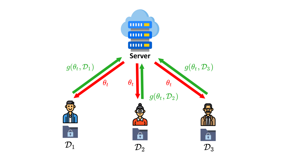
<p>To this end, the optimization is carried out in communication rounds. In particular, given the global parameters $\theta_t$ at round $t$, multiple clients compute model updates $g$ on their own data and then share them with a central server that aggregates them and produces a new global parameters $\theta_{t+1}$. After several communication rounds the model parameters converge to an optimum.
<img src="/assets/blog/lamp/server.svg" class="blogpost-img100" style="height: 500pt;margin: -50pt 0pt -50pt 0pt;" />
One common implementation of this generic framework is the FedSGD algorithm, where updates are given by the gradient of $l$ w.r.t. $\theta_t$ on a single batch $\{(x^b_i, y^b_i)\}\sim \mathcal{D}_i$ of client data of size $B$:</p>
\[\begin{equation*}
  g(\theta_t,\mathcal{D}_i) =  \frac{1}{B} \sum_{b=1}^B \nabla_\theta \left[ l(h_{\theta_t}(x^b_i), y^b_i) \right].
\end{equation*}\]

<p>Federated learning in theory allows for improved data privacy, as the client data does not leave the individual clients. Unfortunately, several recent works have shown that updates $g$ computed by common federated algorithms such as FedSGD can be used by a malicious server during the aggregation phase to approximately reconstruct the client’s data. So far, prior work has focused on exposing this issue in the image domain where strong image priors help the reconstruction. In this work, we show that such approximate reconstruction is also possible in the text domain, where federated learning is very commonly applied.</p>

<h3 id="gradient-leakage">Gradient leakage</h3>

<p>In order to obtain approximate input reconstructions $\{\tilde{x}^b_i\}$ from the FedSGD update of some client $i$, with updates as described above, prior works typically solve the following optimization problem at some communication round $t$:</p>

\[\begin{equation}
  \min_{\\{\tilde{x}^b_i\\}} \sum_{i=1}^n \mathcal{L}_{rec}\left( \left(\frac{1}{B} \sum_{b=1}^B \nabla_\theta l(h_\theta(\tilde{x}^b_i), y^b_i)\right), g(\theta_t, \mathcal{D}_i) \right) + \alpha_{rec}\,R(\{\tilde{x}^b_i\}),
\end{equation}\]

<p>where $\mathcal{L}$<sub>rec</sub> is distance metric - e.g., $L_1$, $L_2$ or cosine, that measures the gradient reconstruction error, $R(\{\tilde{x}^b_i\})$ is some domain specific prior - e.g. Total Variation (TV) in the image domain, that assesses the quality of the reconstructed inputs, and $\alpha_{rec}$ is hyperparameter balancing between the two. Note that $\theta_t$ and $g(\theta_t, \mathcal{D}_i)$ are known by the malicious server as the former is computed by it and the latter is sent to it by client $i$ at the end of the round. Often the batch labels $\{y^b_i\}$ can be obtained by the server using specific label reconstruction attacks, that are beyond the scope of this blog post, or just guessed by running the reconstruction with all possible labels due to their discrete nature, so throughout the post we only focus on reconstructing $\{\tilde{x}^b_i\}$. In <a href="https://www.sri.inf.ethz.ch/blog/bayesian">our previous blog post</a>, we have shown that solving the optimization problem above is equivalent to finding the Bayesian optimal adversary in this setting.</p>

<p>In the image domain, the optimization problem is typically solved using gradient descent on the batch of randomly initialized images $\{x^b_i\}$ using an image-specific prior $R$. In the next section, we first discuss why such a solution is not well suited to language data and we then discuss our method, <strong>LAMP</strong>, that combines a text-specific prior with a new way to solve the optimization problem above by alternating discrete and continuous optimization steps to obtain our state-of-the-art gradient leakage framework for text.</p>

<h3 id="lamp-gradient-leakage-for-text">LAMP: Gradient leakage for text</h3>

<p>In this work, we focus our attention on transformer-based models $h_\theta$, as they are the state-of-the-art for modeling text across various language tasks. As these models operate on continuous vectors, typically they assume fixed-size vocabulary of size $V$ and embed each word into a different $\mathbb{R}^d$ vector. For a sequence of words of size $n$, we refer to the individual words in it with $t_1,\ldots,t_n$ and to their corresponding embeddings with $x_1,\ldots,x_n$.</p>

<p>In order to solve the gradient leakage optimization problem from the previous section, we choose to optimize directly over the embeddings $x_i$ as they, similarly to images, are represented by continuous values we can optimize over. However, uniquely to the text domain, only a finite subset of vectors in $\mathbb{R}^d$ are valid word embeddings. To this end, when we obtain our reconstructed embeddings $\tilde{x}_i$ for each of them we then select the most similar in cosine similarity token in the vocabulary to create a reconstruction of the sequence of words $\tilde{t}_1,\ldots,\tilde{t}_n$.</p>

<p>An additional issue that is specific to the text domain and, in particular, the transformer architecture is that the transformer outputs depend on word order only through positional embeddings. Therefore, the model gradient reconstruction loss $\mathcal{L}$<sub>rec</sub> is not as affected by wrongly reconstructed word order as it is by the wrongly reconstructed word embeddings themselves. In practice, this results into the continuous optimization process often getting stuck in local minima caused by an embedding of a token that reconstructs the correct word at the wrong position. These local minima are hard to escape from continuously.  To this end, we introduce a discrete optimization step that reorders the sentence periodically, allowing to escape the local minima. The discrete step works by first proposing several word order changes such as swapping the positions of two words or moving a sentence prefix to the end of the sentence. The different order changes are then assessed based on the combination of the gradient reconstruction $\mathcal{L}$<sub>rec</sub> and the perplexity of the sentence $\mathcal{L}$<sub>lm</sub> computed by auxiliary language model such as GPT-2 on the projected words $\tilde{t}_i$:</p>

\[\begin{equation}
  \mathcal{L}_{rec}(\{\tilde{x}_i\}) + \alpha_{lm}\,\mathcal{L}_{rec}(\{\tilde{t}_i\}),
\end{equation}\]

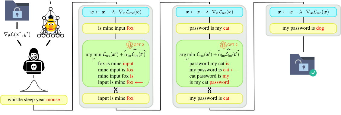
<p>where $\alpha_{lm}$ is a hyperparameter balancing the two parts. The resulting end-to-end alternating optimization is demonstrated in the image below:
<img src="/assets/blog/lamp/lamp.svg" class="blogpost-img100" style="height: 500pt;margin: -100pt 0pt -100pt 0pt;" />
where green boxes show the discrete optimization steps and the blue boxes demonstrate the continuous gradient descent optimization steps of the gradient leakage objective presented in the previous section.</p>
<p>Finally, similarly to the image domain, we introduce a new prior specific to text that improves our reconstruction. To this end, we made the empirical observation that during optimization often the embedding vectors $x_i$ grow in length even when their direction doesn’t change a lot. To this end, we regularize the average vector length of the embeddings in a sequence $\tilde{x}_i$ to be close to the average embedding length in the vocabulary $l_e$:</p>

\[\begin{equation}
  R(\tilde{x}_i) = \left(\frac{1}{n}\sum_{i=1}^n \| \tilde{x}_i \|_2  - l_e\right)^2
\end{equation}\]

<p>This allows our embeddings to remain in the correct range of values, which in turn results in a more stable and accurate reconstruction of the embeddings $\tilde{x}_i$.</p>

<h3 id="experimental-evaluation">Experimental evaluation</h3>

<p>We evaluated LAMP on several standard sentiment classification datasets and architectures based on the BERT language models. As is typically the case with language models, we assume our models are pretrained to make word predictions on large text corpora and that federated learning is used only to fine-tune the models on the classification task at hand. We consider two versions of LAMP - one where $\mathcal{L}$<sub>rec</sub> is a weighted sum of L1 and L2 distances (denoted LAMP<sub>L1+L2</sub>), and another one where $\mathcal{L}$<sub>rec</sub> is the cosine similarity (denoted LAMP<sub>cos</sub>). We compare them to the state-of-the-art attacks - TAG based on the same L1+L2 distance, and DLG based on L2 distance alone. We evaluate the methods in terms of the Rouge-1 metric (R1) which measures the percentage of correctly reconstructed words and the Rouge-2 metric (R2) which measures the percentage of correctly reconstructed bigrams. We note one can interpret R2 as a proxy measurement of how well the order of the sentence has been reconstructed. We present a subset of the results shown in our paper on the CoLA dataset and batch size of 1 below:
<br /><br /></p>
<table>
  <thead>
    <tr>
      <th>&nbsp;</th>
      <th style="text-align: center;" colspan="2">&nbsp;&nbsp;&nbsp;&nbsp;<span style="border-bottom:1px solid black">&nbsp;&nbsp;$\text{TinyBERT}_6$&nbsp;&nbsp;</span>&nbsp;&nbsp;&nbsp;&nbsp;</th>
      <th style="text-align: center;" colspan="2">&nbsp;&nbsp;&nbsp;&nbsp;<span style="border-bottom:1px solid black">&nbsp;&nbsp;$\text{BERT}_{BASE}$&nbsp;&nbsp;</span>&nbsp;&nbsp;&nbsp;&nbsp;</th>
      <th style="text-align: center;" colspan="2">&nbsp;&nbsp;&nbsp;&nbsp;<span style="border-bottom:1px solid black">&nbsp;&nbsp;$\text{BERT}_{LARGE}$&nbsp;&nbsp;</span>&nbsp;&nbsp;&nbsp;&nbsp;</th>
    </tr>
    <tr>
      <th>Method</th>
      <th style="text-align: center">R1</th>
      <th style="text-align: center">R2</th>
      <th style="text-align: center">R1</th>
      <th style="text-align: center">R2</th>
      <th style="text-align: center">R1</th>
      <th style="text-align: center">R2</th>
    </tr>
  </thead>
  <tbody>
    <tr>
      <td>DLG</td>
      <td style="text-align: center">37.7</td>
      <td style="text-align: center">3.0</td>
      <td style="text-align: center">59.3</td>
      <td style="text-align: center">7.7</td>
      <td style="text-align: center">82.7</td>
      <td style="text-align: center">10.5</td>
    </tr>
    <tr>
      <td>TAG</td>
      <td style="text-align: center">43.9</td>
      <td style="text-align: center">3.8</td>
      <td style="text-align: center">78.9</td>
      <td style="text-align: center">10.2</td>
      <td style="text-align: center">82.9</td>
      <td style="text-align: center">14.6</td>
    </tr>
    <tr>
      <td>$\text{LAMP}_{\cos}$</td>
      <td style="text-align: center">93.9</td>
      <td style="text-align: center"><strong>59.3</strong></td>
      <td style="text-align: center"><strong>89.6</strong></td>
      <td style="text-align: center"><strong>51.9</strong></td>
      <td style="text-align: center"><strong>92.0</strong></td>
      <td style="text-align: center"><strong>56.0</strong></td>
    </tr>
    <tr>
      <td>$\text{LAMP}_{\text{L1}+\text{L2}}$</td>
      <td style="text-align: center"><strong>94.5</strong></td>
      <td style="text-align: center">52.1</td>
      <td style="text-align: center">87.5</td>
      <td style="text-align: center">47.5</td>
      <td style="text-align: center">91.2</td>
      <td style="text-align: center">47.8</td>
    </tr>
  </tbody>
</table>
<p><br /><br />
We see that LAMP<sub>cos</sub> is consistently recovering more words compared to the alternatives with LAMP<sub>L1+L2</sub> close behind. Further, LAMP recovers substantially better sentence ordering. It is worth noting that the improvement over the baselines for both R1 and R2 is most pronounced on the smallest model $\text{TinyBERT}_6$ where recovery is the hardest. Additionally, we also experimented with recovering text in the setting where the batch size is bigger than 1. We are the first to present results in this setting and we show them below for the CoLA dataset:
<br /><br /></p>
<table>
  <thead>
    <tr>
      <th>&nbsp;</th>
      <th style="text-align: center;" colspan="2">&nbsp;&nbsp;&nbsp;&nbsp;<span style="border-bottom:1px solid black">&nbsp;&nbsp;&nbsp;&nbsp;&nbsp;&nbsp;B=1&nbsp;&nbsp;&nbsp;&nbsp;&nbsp;&nbsp;</span>&nbsp;&nbsp;&nbsp;&nbsp;</th>
      <th style="text-align: center;" colspan="2">&nbsp;&nbsp;&nbsp;&nbsp;<span style="border-bottom:1px solid black">&nbsp;&nbsp;&nbsp;&nbsp;&nbsp;&nbsp;B=2&nbsp;&nbsp;&nbsp;&nbsp;&nbsp;&nbsp;</span>&nbsp;&nbsp;&nbsp;&nbsp;</th>
      <th style="text-align: center;" colspan="2">&nbsp;&nbsp;&nbsp;&nbsp;<span style="border-bottom:1px solid black">&nbsp;&nbsp;&nbsp;&nbsp;&nbsp;&nbsp;B=4&nbsp;&nbsp;&nbsp;&nbsp;&nbsp;&nbsp;</span>&nbsp;&nbsp;&nbsp;&nbsp;</th>
    </tr>
    <tr>
      <th>Method</th>
      <th style="text-align: center">R1</th>
      <th style="text-align: center">R2</th>
      <th style="text-align: center">R1</th>
      <th style="text-align: center">R2</th>
      <th style="text-align: center">R1</th>
      <th style="text-align: center">R2</th>
    </tr>
  </thead>
  <tbody>
    <tr>
      <td>DLG</td>
      <td style="text-align: center">59.3</td>
      <td style="text-align: center">7.7</td>
      <td style="text-align: center">49.7</td>
      <td style="text-align: center">5.7</td>
      <td style="text-align: center">37.6</td>
      <td style="text-align: center">1.7</td>
    </tr>
    <tr>
      <td>TAG</td>
      <td style="text-align: center">78.9</td>
      <td style="text-align: center">10.2</td>
      <td style="text-align: center">68.8</td>
      <td style="text-align: center">7.6</td>
      <td style="text-align: center">56.2</td>
      <td style="text-align: center">6.7</td>
    </tr>
    <tr>
      <td>$\text{LAMP}_{\cos}$</td>
      <td style="text-align: center"><strong>89.6</strong></td>
      <td style="text-align: center"><strong>51.9</strong></td>
      <td style="text-align: center">74.4</td>
      <td style="text-align: center">29.5</td>
      <td style="text-align: center">55.2</td>
      <td style="text-align: center">14.5</td>
    </tr>
    <tr>
      <td>$\text{LAMP}_{\text{L1}+\text{L2}}$</td>
      <td style="text-align: center">87.5</td>
      <td style="text-align: center">47.5</td>
      <td style="text-align: center"><strong>78.0</strong></td>
      <td style="text-align: center"><strong>31.4</strong></td>
      <td style="text-align: center"><strong>66.2</strong></td>
      <td style="text-align: center"><strong>21.8</strong></td>
    </tr>
  </tbody>
</table>
<p><br /><br />
We see that despite the worse quality of reconstruction, even batch size of 4 still leaks a substantial amount of data. Further, we observe that for bigger batch sizes LAMP<sub>L1+L2</sub> performs better than LAMP<sub>cos</sub>. Both LAMP methods, however, substantially improve upon the results of the baselines.
Finally, we show an example sentence reconstruction from LAMP and TAG on multiple datasets below:
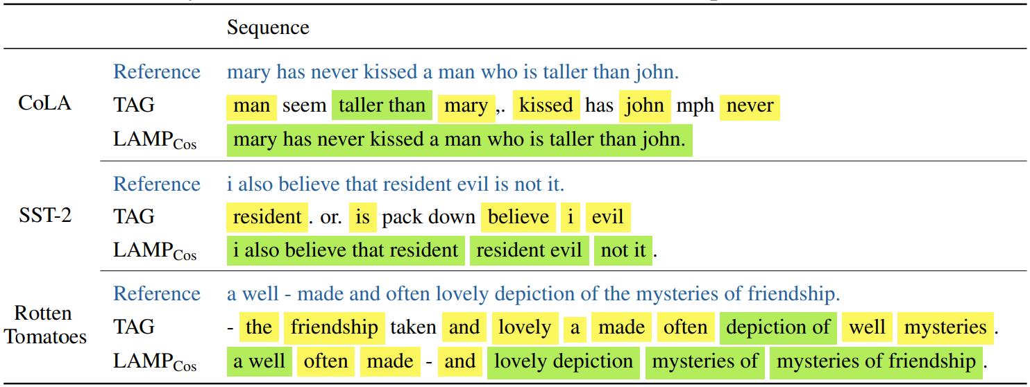
<img src="/assets/blog/lamp/text_rec.png" class="blogpost-img100" style="margin: 30pt 0pt 30pt 0pt;" />
Here, yellow signifies a single correctly reconstructed word and green signifies a tuple of correctly recovered words. We see that LAMP recovers the word order drastically better and often is even able to reconstruct it perfectly. In addition, LAMP recovers more individual words. This confirms qualitatively the effectiveness of our attack.</p>
<h3 id="summary">Summary</h3>

<p>In this blog post, we introduced LAMP, a new framework for gradient leakage of text data from gradient updates in federated learning. Our key ideas are the alternating of continuous and discrete optimization steps and the introduction of an auxiliary text model which we use in the discrete part of our optimization to judge how well a piece of text is reconstructed. Thanks to these elements, our attack is able to produce substantially better text reconstructions compared to the state-of-the-art attacks both quantitatively and qualitatively. We, thus, show that many practical federated learning systems based on text are vulnerable and better mitigation steps should be taken.
For more details please see our <a href="https://files.sri.inf.ethz.ch/website/papers/balunovic2022lamp.pdf">NeurIPS 2022 paper</a>.</p>]]></content><author><name></name></author><category term="paper" /><summary type="html"><![CDATA[In this work we present an attack on federated learning's privacy specific to the text domain. We show that federated learning in the text domain can expose a lot of user data.]]></summary></entry><entry><title type="html">Reliability Guarantees on Private Data</title><link href="https://www.sri.inf.ethz.ch/blog/phoenix" rel="alternate" type="text/html" title="Reliability Guarantees on Private Data" /><published>2022-11-07T00:00:00+00:00</published><updated>2022-11-07T00:00:00+00:00</updated><id>https://www.sri.inf.ethz.ch/blog/phoenix</id><content type="html" xml:base="https://www.sri.inf.ethz.ch/blog/phoenix"><![CDATA[<p>In this post we present our ACM CCS 2022 publication, <a href="https://www.sri.inf.ethz.ch/publications/jovanovic2022phoenix">Private and Reliable Neural Network Inference</a>, where we introduced Phoenix, a tool for NN inference that both protects client data privacy and enables important reliability guarantees.</p>

<p>We focus on the common <em>ML as a service</em> scenario, a two-party setting where a client offloads intensive computation (commonly NN inference) to the server.
The client data is of sensitive nature in many of the applications (e.g., financial, judicial), which motivated work in the field of <em>privacy-preserving NN inference</em>, aiming to build methods that perform the computation without the server learning the client data. 
One of the most common techniques for this is  <em>fully-homomorphic encryption</em> (FHE), which is rapidly becoming more practical.</p>

<p>Orthogonal to privacy, a long line of work focuses on enabling <em>NN inference with reliability guarantees</em>.
For example, in a loan prediction setting, augmenting predictions with <em>fairness</em> guarantees is in the interest of both parties, as it increases trust in the system and may be essential to ensure regulatory compliance.
Some of the latest works in this direction are <a href="https://www.sri.inf.ethz.ch/publications/peychev2022latent">LASSI</a> and <a href="https://www.sri.inf.ethz.ch/publications/jovanovic2023fare">FARE</a>, focusing on two aspects of the fairness problem.
Another common example is <em>robustness</em>, where for example, a medical image analysis system should be able to prove to clients that the diagnosis is robust to naturally-occurring measurement errors (see e.g., our latest work <a href="https://openreview.net/forum?id=7oFuxtJtUMH">SABR</a>).</p>

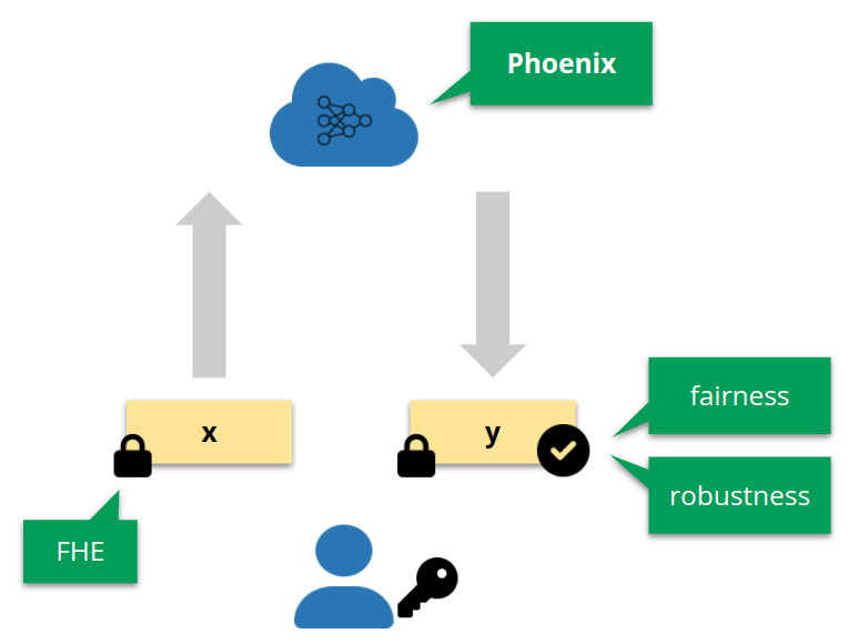
<p><img src="/assets/blog/phoenix/mlaas.png" alt="" class="blogpost-img50" /></p>

<p class="blogpost-caption"><em><strong>ML as a service.</strong> Phoenix achieves both client data privacy (via FHE) and fairness/robustness guarantees.</em></p>

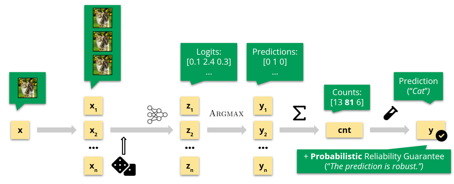
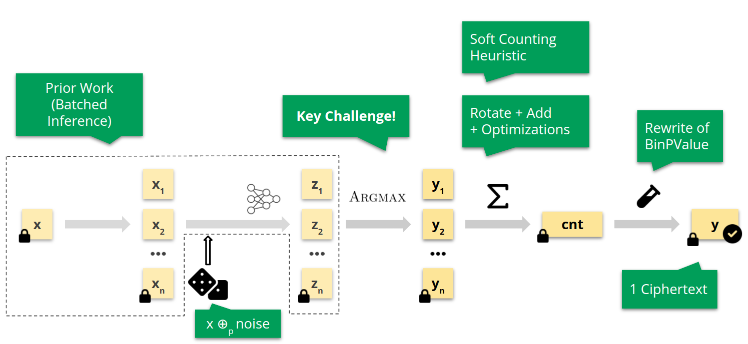
<p>While the problems of privacy-preserving and reliable inference are both well-established, there was no prior attempt to consolidate the work in these two fields.
Thus, service providers who offer reliability guarantees currently have no simple way to transition their service to a privacy-preserving setting, a requirement which is becoming increasingly relevant. 
This is the problem we address in Phoenix, proposing a system that supports both: client data privacy and reliability guarantees.
To this end, we lift the key building blocks of <a href="https://arxiv.org/abs/1902.02918">randomized smoothing</a>, a technique for augmenting predictions with reliability guarantees, to the popular <a href="https://eprint.iacr.org/2016/421.pdf">RNS-CKKS</a> FHE scheme.
The key challenges that Phoenix overcomes stem from the missing native support for control flow and evaluation of non-polynomial functions in the FHE scheme.</p>

<p>We now recall randomized smoothing on a high level.</p>

<p><img src="/assets/blog/phoenix/smoothing.png" alt="" class="blogpost-img100" /></p>

<p class="blogpost-caption"><em><strong>Randomized smoothing.</strong> A high-level overview of the procedure in the non-private setting.</em></p>

<p>As the service provider, we receive an input $x$ (in the illustration above, a cat image), and we aim to return a prediction $y$ (for some classification task) augmented with a reliability guarantee, for a property such as robustness.
We duplicate the input $n$ times, add independently sampled Gaussian noise to each copy, and perform batched NN inference to obtain the logit vectors, i.e., unnormalized probabilities.
Next, we apply the Argmax function to transform logits to predictions, and aggregate those predictions across $n$ samples to get the <em>counts</em>, indicating how many times each output class was predicted.
Finally, we perform a statistical test on the counts, which, if successful, produces a probabilistic reliability guarantee, ensuring that the prediction $y$ is robust with known high probability.</p>

<p>The key question is how this procedure needs to change if we attempt to execute it while protecting client data privacy, i.e., if the data is encrypted using FHE by the client.
The key steps are illustrated below.</p>

<p><img src="/assets/blog/phoenix/phoenix.png" alt="" class="blogpost-img100" /></p>

<p class="blogpost-caption"><em><strong>Overview of Phoenix.</strong> The main challenges in lifting randomized smoothing to FHE.</em></p>

<p>For the batched NN inference (dashed line) we directly utilize prior work, which offers efficient algorithms for the RNS-CKKS scheme. 
Further, the addition of noise is simple, as the noise can be directly added as a plaintext due to the homomorphic property.
However, computing Argmax is a key challenge due to the difficulty of computing non-polynomial functions—we elaborate on this shortly.
In the aggregation step we combine several methods from prior work with scheme-specific optimizations, and develop a novel heuristic for randomized smoothing, necessary to obtain a computationally feasible procedure.
Finally, we perform a rewrite of the one-sided binomial test applied to counts to make it FHE-suitable.
The output of Phoenix is a single ciphertext, which when decrypted with the secret key of the client, reveals both the prediction and the computed reliability guarantee.
We next discuss the Argmax approximation in more detail, and refer to our paper for details regarding all other steps.</p>

<p class="blogpost-wrap"><img src="/assets/blog/phoenix/argmax.png" alt="" class="blogpost-img20" />
<span>
To efficiently approximate Argmax, we use the recent paper of <a href="https://eprint.iacr.org/2019/1234">Cheon et al. (ASIACRYPT ‘20)</a>, which propose <em>SgnHE</em>, a sign function approximation for FHE as a composition of low-degree polynomials, illustrated below.
Our approximate Argmax is built on several applications of <em>SgnHE</em> (see the paper for the full algorithm).
Most importantly, in our case it is crucial to have guarantees on the approximation quality of <em>SgnHE</em>—otherwise, the randomized smoothing reliability guarantee returned to the clients may in some cases be invalid, fundamentally compromising the protocol.
<span></span></span></p>

<p><img src="/assets/blog/phoenix/sgn.png" alt="" class="blogpost-img50" /></p>

<p class="blogpost-caption"><em><strong>Sign function approximation.</strong> Repeated applications of the polynomial $f_0$ increase approximation quality.</em></p>

<p>The <em>SgnHE</em> function is parametrized such that for desired parameters $a,b \in \mathbb{R}$, we can obtain an $(a,b)$-close approximation, meaning that for inputs $x \in [a, 1]$ the output is guaranteed to be in $[1 - 2^{-b}, 1]$ (similarly for the negative case). 
However, as the server is unable to directly observe the intermediate values due to encryption, it is hard to ensure the above precondition is satisfied for logit values which are the input to the Argmax, and the first of the sign function applications it utilizes.</p>

<p>To overcome this we impose two <em>conditions</em> on the logit vectors, constraining the range and differences of their values, allowing us to appropriately rescale them and reason about the approximation quality.
As we can not prove for an arbitrary NN that such conditions on logits will always hold (e.g., be in some range), we use confidence intervals and a finite sample to upper bound the condition violation probability. 
When reporting the guarantee to the client, the computed probability (approximation error) is added to the usual error probability of randomized smoothing as the probabilistic procedure (algorithmic error).
The resulting value represents the total error probability of our guarantee, maintaining the behavior of the non-private case.</p>

<p>In our extensive experiments across multiple scenarios we observe values for the total error probability of around 1%, confirming that our procedure leads to viable high-probability guarantees.
We further observe non-restrictive latencies and communication cost and high <em>consistency</em>, i.e., the results obtained with the FHE version of randomized smoothing are in almost 100% of the cases identical to those of the non-private baseline, confirming that transitioning a service to FHE using Phoenix does not sacrifice the key metrics.
Our Microsoft SEAL implementation is publicly available on <a href="https://github.com/eth-sri/phoenix">GitHub</a>.</p>

<p>We believe Phoenix is an important first step towards merging the worlds of reliable and privacy-preserving machine learning.
For more details of the Argmax approximation, omitted parts of the protocol, as well as detailed experimental results including microbenchmarks, please refer to our paper.</p>]]></content><author><name></name></author><category term="paper" /><summary type="html"><![CDATA[We present Phoenix (CCS '22), the first system for privacy-preserving neural network inference with robustness and fairness guarantees.]]></summary></entry><entry><title type="html">Why Tighter Convex Relaxations Harm Certified Training</title><link href="https://www.sri.inf.ethz.ch/blog/paradox" rel="alternate" type="text/html" title="Why Tighter Convex Relaxations Harm Certified Training" /><published>2022-10-27T00:00:00+00:00</published><updated>2022-10-27T00:00:00+00:00</updated><id>https://www.sri.inf.ethz.ch/blog/paradox</id><content type="html" xml:base="https://www.sri.inf.ethz.ch/blog/paradox"><![CDATA[<p>This blog post summarizes the key findings of our paper <a href="https://www.sri.inf.ethz.ch/publications/jovanovic2022paradox">On the Paradox Of Certified Training</a>, which was recently published in TMLR.</p>

<p>We attempt to explain the phenomenon where most state-of-the-art methods for certified training based on convex relaxations (such as <a href="https://proceedings.neurips.cc/paper/2021/hash/988f9153ac4fd966ea302dd9ab9bae15-Abstract.html">FastIBP</a> or the latest breakthrough <a href="https://openreview.net/forum?id=7oFuxtJtUMH">SABR</a>) focus on the loose interval propagation (IBP/Box), while intuitively, tighter relaxations (i.e., the ones that more tightly overapproximate the non-linearities in the network) should lead to better results. 
This was <a href="https://arxiv.org/abs/1810.12715">already</a> <a href="https://www.ijcai.org/proceedings/2019/854">observed</a> <a href="https://openreview.net/forum?id=Skxuk1rFwB">in</a> <a href="https://www.sri.inf.ethz.ch/publications/balunovic2020bridging">many</a> <a href="https://arxiv.org/abs/2104.00447">prior</a> <a href="https://openreview.net/forum?id=52weXyh2yh">works</a>, which proposed several hypotheses. However, the paradox was never investigated in a principled way.</p>

<p>We start by proposing a way to quantify tightness (see the paper for details), and thoroughly reproducing the paradox: Across a wide range of settings, tighter relaxations consistently lead to lower certified robustness (in %) than the loose IBP relaxation. An example is shown in the following table, grouping equivalent methods from prior work (below we will refer to each group using the name in bold):</p>

<style>
    .good {
        background-color: #aaffaa;
        padding: 1px;
        width: 40px;
        display: inline-block;
    }
    .bad {
        background-color: #ffaaaa;
        padding: 1px;
        width: 40px;
        display: inline-block;
    }
</style>

<table>
  <thead>
    <tr>
      <th>Relaxation</th>
      <th style="text-align: center">Tightness</th>
      <th style="text-align: center">Certified (%)</th>
    </tr>
  </thead>
  <tbody>
    <tr>
      <td><strong>IBP</strong> / Box</td>
      <td style="text-align: center"><span class="bad"> 0.73 </span></td>
      <td style="text-align: center"><span class="good"> 86.8 </span></td>
    </tr>
  </tbody>
  <tbody>
    <tr>
      <td><strong>hBox</strong> / Symbolic Intervals</td>
      <td style="text-align: center"><span class="good"> 1.76 </span></td>
      <td style="text-align: center"><span class="bad"> 83.7 </span></td>
    </tr>
    <tr>
      <td><strong>CROWN</strong> / DeepPoly</td>
      <td style="text-align: center"><span class="good"> 3.36 </span></td>
      <td style="text-align: center"><span class="bad"> 70.2 </span></td>
    </tr>
    <tr>
      <td><strong>DeepZ</strong> / CAP / FastLin / Neurify</td>
      <td style="text-align: center"><span class="good"> 3.00 </span></td>
      <td style="text-align: center"><span class="bad"> 69.8 </span></td>
    </tr>
    <tr>
      <td><strong>CROWN-IBP (R)</strong></td>
      <td style="text-align: center"><span class="good"> 2.15 </span></td>
      <td style="text-align: center"><span class="bad"> 75.4 </span></td>
    </tr>
  </tbody>
</table>

<p>Our key observation is that there are other latent properties of relaxations, besides tightness, that affect success when relaxations are used in a training procedure.
More concretely, each of the tighter relaxations has either unfavorable <em>continuity</em> (i.e., the corresponding loss function is discontinuous with respect to network weights) or unfavorable <em>sensitivity</em> (i.e., the corresponding loss function is highly sensitive to small perturbations of network weights), both preventing successful optimization. By observing all three properties jointly, we can more easily interpret the seemingly counterintuitive results.</p>

<p>The plot below shows the relaxation of the ReLU non-linearity used by CROWN, for the example input range defined by $l=-5$ and $u=8$. By reducing $u$ (using the bottom slider), we can directly observe the discontinuity of CROWN, when its heuristic choice of the lower linear bound changes at $|l|=|u|$. Using the same plot we can observe the discontinuities of hBox at $l=0$. 
These observations imply discontinuities in the loss when a relaxation is used in training, which we further empirically observe in real scenarios.
Finally, we can use the plot below to observe that no discontinuities can be found for IBP and DeepZ—a formal proof of their continuity in the general case is given in the paper.</p>

<p><a class="iframe-link" href="/assets/blog/paradox/continuity.html"> Open Interactive Plot</a></p>

<iframe class="iframe-full" src="/assets/blog/paradox/continuity.html" height="780px"></iframe>

<p>While the sensitivity of the loss functions is harder to illustrate on a toy example as above, our derivation (Section 4.3 of the paper) demonstrates that the bounds used by CROWN, CROWN-IBP (R) and DeepZ lead to certified training losses highly sensitive to small changes in network weights, while the losses of IBP and hBox are not sensitive and induce more favorable loss landscapes. With these observations, we expand the table shown earlier to include all three relaxation properties: tightness, continuity and sensitivity. 
This illustrates that attempts to use tighter relaxations in certified training have introduced unfavorable properties of the loss, which resulted in the failure to outperform the continuous and non-sensitive IBP.</p>

<table>
  <thead>
    <tr>
      <th>Relaxation</th>
      <th style="text-align: center">Tightness</th>
      <th style="text-align: center">Continuity</th>
      <th style="text-align: center">Sensitivity</th>
      <th style="text-align: center">Certified (%)</th>
    </tr>
  </thead>
  <tbody>
    <tr>
      <td><strong>IBP</strong> / Box</td>
      <td style="text-align: center"><span class="bad"> 0.73 </span></td>
      <td style="text-align: center"><span class="good"> $\checkmark$ </span></td>
      <td style="text-align: center"><span class="good"> $\checkmark$ </span></td>
      <td style="text-align: center"><span class="good"> 86.8 </span></td>
    </tr>
  </tbody>
  <tbody>
    <tr>
      <td><strong>hBox</strong> / Symbolic Intervals</td>
      <td style="text-align: center"><span class="good"> 1.76 </span></td>
      <td style="text-align: center"><span class="bad"> $\times$ </span></td>
      <td style="text-align: center"><span class="good"> $\checkmark$ </span></td>
      <td style="text-align: center"><span class="bad"> 83.7 </span></td>
    </tr>
    <tr>
      <td><strong>CROWN</strong> / DeepPoly</td>
      <td style="text-align: center"><span class="good"> 3.36 </span></td>
      <td style="text-align: center"><span class="bad"> $\times$ </span></td>
      <td style="text-align: center"><span class="bad"> $\times$ </span></td>
      <td style="text-align: center"><span class="bad"> 70.2 </span></td>
    </tr>
    <tr>
      <td><strong>DeepZ</strong> / CAP / FastLin / Neurify</td>
      <td style="text-align: center"><span class="good"> 3.00 </span></td>
      <td style="text-align: center"><span class="good"> $\checkmark$ </span></td>
      <td style="text-align: center"><span class="bad"> $\times$ </span></td>
      <td style="text-align: center"><span class="bad"> 69.8 </span></td>
    </tr>
    <tr>
      <td><strong>CROWN-IBP (R)</strong></td>
      <td style="text-align: center"><span class="good"> 2.15 </span></td>
      <td style="text-align: center"><span class="bad"> $\times$ </span></td>
      <td style="text-align: center"><span class="bad"> $\times$</span></td>
      <td style="text-align: center"><span class="bad"> 75.4 </span></td>
    </tr>
  </tbody>
</table>

<h3 id="next-steps">Next steps</h3>

<p>A natural question that arises is the one of improving unfavorable properties of relaxations to make them more suitable for certified training. 
In the paper we systematically investigate modifications of existing relaxations and find that designing a relaxation with all favorable properties is difficult, as the properties induce complex tradeoffs that depend on the setting. 
Still, such relaxations may exist, and future work might be able to utilize our findings to discover them.</p>

<p>A more promising approach seems to be the use of existing convex relaxations with modified training procedures designed to best utilize the benefits of each relaxation. Recent successful examples of this approach include <a href="https://www.sri.inf.ethz.ch/publications/balunovic2020bridging">COLT</a>, which includes the counterexample search in training, <a href="https://openreview.net/forum?id=Skxuk1rFwB">CROWN-IBP</a>, which heuristically combines the losses of two relaxations in training, and two recent methods which focus on IBP, aiming to improve its training procedure via better initialization and regularization (<a href="https://proceedings.neurips.cc/paper/2021/hash/988f9153ac4fd966ea302dd9ab9bae15-Abstract.html">FastIBP</a>) or the propagation of 
smaller input regions in training (<a href="https://openreview.net/forum?id=7oFuxtJtUMH">SABR</a>).</p>

<p>Finally, it is worth noting that there are other promising approaches for neural network certification that do not use convex relaxations and are thus not affected by tradeoffs between relaxation properties. Examples in this direction include <a href="https://arxiv.org/abs/1902.02918">Randomized Smoothing</a>, offering high-probability robustness certificates, and custom certification-friendly model architectures such as <a href="https://arxiv.org/abs/2102.05363">$l_\infty$-distance nets</a>. 
While not affected by limitations of convex relaxations, these approaches introduce other challenges such as optimization difficulties and additional inference-time work.</p>]]></content><author><name></name></author><category term="paper" /><summary type="html"><![CDATA[We investigate a long-standing paradox in the field of certified training, identifying previously overlooked properties of convex relaxations which affect training success.]]></summary></entry><entry><title type="html">SRI Lab at ICLR 2022</title><link href="https://www.sri.inf.ethz.ch/blog/iclr2022" rel="alternate" type="text/html" title="SRI Lab at ICLR 2022" /><published>2022-04-25T00:00:00+00:00</published><updated>2022-04-25T00:00:00+00:00</updated><id>https://www.sri.inf.ethz.ch/blog/iclr2022</id><content type="html" xml:base="https://www.sri.inf.ethz.ch/blog/iclr2022"><![CDATA[]]></content><author><name></name></author><category term="meta" /><summary type="html"><![CDATA[SRI Lab will present five works at ICLR 2022! In this meta post we aggregate all content related to our ICLR papers, including links to the conference portal and individual blogposts where you can learn more about the topics we currently focus on.]]></summary><media:thumbnail xmlns:media="http://search.yahoo.com/mrss/" url="https://www.sri.inf.ethz.ch/assets/blog/fb_preview/iclr.jpg" /><media:content medium="image" url="https://www.sri.inf.ethz.ch/assets/blog/fb_preview/iclr.jpg" xmlns:media="http://search.yahoo.com/mrss/" /></entry><entry><title type="html">Generating Provably Robust Adversarial Examples</title><link href="https://www.sri.inf.ethz.ch/blog/parade" rel="alternate" type="text/html" title="Generating Provably Robust Adversarial Examples" /><published>2022-04-21T00:00:00+00:00</published><updated>2022-04-21T00:00:00+00:00</updated><id>https://www.sri.inf.ethz.ch/blog/parade</id><content type="html" xml:base="https://www.sri.inf.ethz.ch/blog/parade"><![CDATA[<p><img src="/assets/blog/parade/motivation.svg" class="blogpost-img100" style="height: 200pt;" />
On the image above we show an image of the digit $0$ from MNIST ($x_\text{orig}$) and a region around it in red that depicts the set of geometrically perturbed images for which we expect a given neural network to be robust. 
Further, in green we depict a subregion where the neural network is not robust. Traditionally, in order to assess the robustness of the network one uses adversarial attacks to generate the examples $x_1$ and $x_2$. 
While robustness can be assessed that way, the information that the whole green region is adversarial is lost. This in turn might lead to never-seen-before network behaviour in the future. 
One advantage of the classical approach of assessing robustness, however,  is that generating $x_1$ and $x_2$ is fast. In contrast, generating the green region is computationally infeasible.
In this work, we present an algorithm called <strong>PARADE</strong> that exploits classical adversarial attacks to generate as large as possible regions that are provably adversarial. Similarly to the green region in the figure, these regions summarize many indvidual advarsarial attacks while also being practical to compute. 
We call them provably robust adversarial examples.</p>

<h3 id="algorithm-overview">Algorithm overview</h3>
<p>There are three main steps to <strong>PARADE</strong>. First, we generate an initial box region that might contain non-adversarial points using off-the-shelf adversarial attacks. 
We refer to this region as the overapproximation box $\mathcal{O}$. Then, we use a black-box verifier to shrink this overapproximation box to a smaller box that provably contains only adversarial points. We call this region the underapproximation box $\mathcal{U}$.
Finally, we use  $\mathcal{O}$ and $\mathcal{U}$ to generate a polyhedral region  $\mathcal{U}\subseteq\mathcal{P}\subseteq\mathcal{O}$ that we also prove only contains adversarial points using the same black-box verifier. Both $\mathcal{U}$ and $\mathcal{P}$ fit our definition of 
provably robust adversarial examples but differ in terms of shape and precision. To this end, the generation of $\mathcal{P}$ is only an optional way to make our provably robust adversarial examples more precise. Next, we present the <strong>PARADE</strong> steps in details.</p>

<h3 id="generating-the-overapproximation-box--mathcalo">Generating the overapproximation box  $\mathcal{O}$</h3>
<iframe src="/assets/blog/parade/over.svg" style="border: none;;width: 100%;height: 200pt;"></iframe>
<p>To generate the overapproximation box $\mathcal{O}$, we sample attacks from an adversarial attack algorithm, such as <strong>PGD</strong>. Then, we fit a box around them. The process is illustateted in the animation above. 
We note that depending on the success of the attack algorithm, a small part of the ground truth adversarial region $\mathcal{T}$ might be excluded from $\mathcal{O}$.</p>

<h3 id="generating-the-underapproximation-box--mathcalu">Generating the underapproximation box  $\mathcal{U}$</h3>
<iframe src="/assets/blog/parade/under.svg" style="border: none;;width: 100%;height: 264pt;"></iframe>
<p>We aim to generate the underapproximation box $\mathcal{U}$ in a way that it can be proven to only contain adversarial examples while also being as large as possible. Due to the complexity of this objective, we do this heuristically. In particular, we start by initializing $\mathcal{U}$
to the overapproximation box $\mathcal{O}$. At each iteration $i$, we execute a black-box verification procedure. If the procedure verifies that the box from the previous iteration, $\mathcal{U}_{i-1}$, contains only adversarial examples, we return it. 
Otherwise, we obtain from the verifier a linear contraint, which can be added to $\mathcal{U}_{i-1}$ in order to make it provably robust. Unfortunately, the constraint is usually too conservative, as the black-box verifier relies on overapproximation of the set of possible network outputs. To this end, we relax the constraint by bias-adjusting it.
We make sure that we cannot relax the constraint too much, such that it becomes meaningless. We use the bias-adjusted contraint to shrink $\mathcal{U}_{i-1}$ such that the constraint is not violated but the smallest possible amount of volume is lost. The procedure is repeated until the verification succeeds. The process is depicted in the animation above.</p>

<h3 id="generating-the-polyhedral-region--mathcalp">Generating the polyhedral region  $\mathcal{P}$</h3>
<iframe src="/assets/blog/parade/poly.svg" style="border: none;;width: 100%;height: 240pt;"></iframe>
<p>Finally, we present the optional step of generating polyhedral provably robust adversarial example $\mathcal{P}$ from the box provably robust adversarial example $\mathcal{U}$. 
The additional flexibility of the polyhedral shape allows for larger regions $\mathcal{P}$ compared to $\mathcal{U}$ in exchange for computational complexity. As generating polyhedral regions is hard, we again do this heuristically.
Starting with the overapproximation box $\mathcal{O}$, we iteratively add linear containts to it until we arrive at a polyhedron $\mathcal{P}$ that can be proved to only contain adversarial examples by the black-box verifier. 
Similarly to the generation process of $\mathcal{U}$, we use the verification at iteration $i$ to generate linear contraints. 
Unlike the generation process of $\mathcal{U}$, we use not only linear constraints from the final verification objective but also linear constraints that make the <em>ReLU</em> activation neurons in the network decided. 
Unfortunately, the resulting constraints might generate polyhedron $\mathcal{P}$ that is smaller than $\mathcal{O}$. To prevenet that, we leverage the fact that $\mathcal{U}$ is itself provably robust and we bias-adjust the constraints in such a way that they do not remove volume from $\mathcal{U}$.
The procedure is concludes when the verifier succeeds. We outline the procedure in the animation above.</p>

<h3 id="experiments">Experiments</h3>

<p>We experimented with two different types of provably robust adversarial examples - robust to pixel intensity changes ($\ell_\infty$ changes) and to geometric changes. We show the pixel intensity experiment below:</p>

<table>
  <thead>
    <tr>
      <th>Network</th>
      <th style="text-align: right">$\epsilon$</th>
      <th style="text-align: right">PARADE<br />Box<br /># Regions</th>
      <th style="text-align: right">PARADE<br />Box<br />Time</th>
      <th style="text-align: right">PARADE<br />Box<br /># Attacks</th>
      <th style="text-align: right">PARADE<br />Poly<br /># Regions</th>
      <th style="text-align: right">PARADE<br />Poly<br /> Time</th>
      <th style="text-align: right">PARADE<br />Poly<br /># Attacks</th>
    </tr>
  </thead>
  <tbody>
    <tr>
      <td>MNIST<br />8x200</td>
      <td style="text-align: right">0.045</td>
      <td style="text-align: right">53/53</td>
      <td style="text-align: right">114s</td>
      <td style="text-align: right">$10^{121}$</td>
      <td style="text-align: right">53/53</td>
      <td style="text-align: right">1556s</td>
      <td style="text-align: right">$10^{121} &lt; \cdot &lt; 10^{191}$</td>
    </tr>
    <tr>
      <td>MNIST<br />ConvSmall</td>
      <td style="text-align: right">0.12</td>
      <td style="text-align: right">32/32</td>
      <td style="text-align: right">74s</td>
      <td style="text-align: right">$10^{494}$</td>
      <td style="text-align: right">32/32</td>
      <td style="text-align: right">141s</td>
      <td style="text-align: right">$10^{494} &lt; \cdot &lt; 10^{561}$</td>
    </tr>
    <tr>
      <td>MNIST<br />ConvBig</td>
      <td style="text-align: right">0.05</td>
      <td style="text-align: right">28/29</td>
      <td style="text-align: right">880s</td>
      <td style="text-align: right">$10^{137}$</td>
      <td style="text-align: right">28/29</td>
      <td style="text-align: right">5636s</td>
      <td style="text-align: right">$10^{137} &lt; \cdot &lt; 10^{173}$</td>
    </tr>
    <tr>
      <td>CIFAR-10<br />ConvSmall</td>
      <td style="text-align: right">0.006</td>
      <td style="text-align: right">44/44</td>
      <td style="text-align: right">113s</td>
      <td style="text-align: right">$10^{486}$</td>
      <td style="text-align: right">44/44</td>
      <td style="text-align: right">264s</td>
      <td style="text-align: right">$10^{486} &lt; \cdot &lt; 10^{543}$</td>
    </tr>
    <tr>
      <td>CIFAR-10<br />ConvBig</td>
      <td style="text-align: right">0.008</td>
      <td style="text-align: right">36/36</td>
      <td style="text-align: right">404s</td>
      <td style="text-align: right">$10^{573}$</td>
      <td style="text-align: right">36/36</td>
      <td style="text-align: right">610s</td>
      <td style="text-align: right">$10^{573} &lt; \cdot &lt; 10^{654}$</td>
    </tr>
  </tbody>
</table>

<p>We note <strong>PARADE</strong> is highly effective - it generates regions successfully for all but $1$ image for which the classical adversarial attacks succeeded. Further, the regions generated contain a very large set of adversarial examples that are infeasible to generate individually.
Finally, we note that the polyhedral adversarial examples take more time to generate but contain more examples. Calculating the exact number of concrete attacks within the polyhedral regions is computationally hard so instead we approximate the number as precisely as possible from above and below using boxes.</p>

<p>Next, we show the results for adversarial examples provably robust to geometric changes:</p>

<table>
  <thead>
    <tr>
      <th>Network</th>
      <th style="text-align: right">Transform</th>
      <th style="text-align: right">PARADE<br />Box<br /># Regions</th>
      <th style="text-align: right">PARADE<br />Box<br />Time</th>
      <th style="text-align: right">PARADE<br />Box<br /># Attacks</th>
    </tr>
  </thead>
  <tbody>
    <tr>
      <td>MNIST<br />ConvSmall</td>
      <td style="text-align: right">Rotate + Scale + Shear</td>
      <td style="text-align: right">51/54</td>
      <td style="text-align: right">774s</td>
      <td style="text-align: right">$10^{96} &lt; \cdot &lt; 10^{195}$</td>
    </tr>
    <tr>
      <td>MNIST<br />ConvSmall</td>
      <td style="text-align: right">Scale + Translate2D</td>
      <td style="text-align: right">51/56</td>
      <td style="text-align: right">521s</td>
      <td style="text-align: right">$10^{71} &lt; \cdot &lt; 10^{160}$</td>
    </tr>
    <tr>
      <td>MNIST<br />ConvSmall</td>
      <td style="text-align: right">Scale + Rotate + Brightness</td>
      <td style="text-align: right">40/48</td>
      <td style="text-align: right">370s</td>
      <td style="text-align: right">$10^{70} &lt; \cdot &lt; 10^{455}$</td>
    </tr>
    <tr>
      <td>MNIST<br />ConvBig</td>
      <td style="text-align: right">Rotate + Scale + Shear</td>
      <td style="text-align: right">44/50</td>
      <td style="text-align: right">835s</td>
      <td style="text-align: right">$10^{77} &lt; \cdot &lt; 10^{205}$</td>
    </tr>
    <tr>
      <td>MNIST<br />ConvBig</td>
      <td style="text-align: right">Scale + Translate2D</td>
      <td style="text-align: right">42/46</td>
      <td style="text-align: right">441s</td>
      <td style="text-align: right">$10^{64} &lt; \cdot &lt; 10^{174}$</td>
    </tr>
    <tr>
      <td>MNIST<br />ConvBig</td>
      <td style="text-align: right">Scale + Rotate + Brightness</td>
      <td style="text-align: right">46/52</td>
      <td style="text-align: right">537s</td>
      <td style="text-align: right">$10^{119} &lt; \cdot &lt; 10^{545}$</td>
    </tr>
    <tr>
      <td>CIFAR-10<br />ConvSmall</td>
      <td style="text-align: right">Rotate + Scale + Shear</td>
      <td style="text-align: right">29/29</td>
      <td style="text-align: right">1369s</td>
      <td style="text-align: right">$10^{599} &lt; \cdot &lt; 10^{1173}$</td>
    </tr>
    <tr>
      <td>CIFAR-10<br />ConvSmall</td>
      <td style="text-align: right">Scale + Translate2D</td>
      <td style="text-align: right">32/32</td>
      <td style="text-align: right">954s</td>
      <td style="text-align: right">$10^{66} &lt; \cdot &lt; 10^{174}$</td>
    </tr>
    <tr>
      <td>CIFAR-10<br />ConvSmall</td>
      <td style="text-align: right">Scale + Rotate + Brightness</td>
      <td style="text-align: right">21/25</td>
      <td style="text-align: right">1481s</td>
      <td style="text-align: right">$10^{513} &lt; \cdot &lt; 10^{2187}$</td>
    </tr>
  </tbody>
</table>

<p>We see that again <strong>PARADE</strong> is capable of generating examples for most images where classical adversarial attacks succeeded. We note that we use <a href="https://www.sri.inf.ethz.ch/publications/balunovic2019geometric"><em>DeepG</em></a> for verification. 
Since DeepG generates image polyhedra, we have to approximate the number of concrete attacks similarly to <strong>PARADE Poly</strong> above. We also note that DeepG is more computationally expensive resulting is longer runtime for our algorithm, as well.</p>

<h3 id="visualizing-parade-regions">Visualizing PARADE regions</h3>
<p><img src="/assets/blog/parade/visualize.svg" alt="" class="blogpost-img100" /></p>

<p>Above we visualize some of the provably robust adversarial examples generated by <strong>PARADE</strong> for both pixel and geometric transformations. Each pixel’s color represents the number of possible values that pixel can have within our box regions.</p>
<h3 id="summary">Summary</h3>
<p>We introduced and motivated the concept of provably robust adversarial examples. We further showed an outline of our algorithm, <strong>PARADE</strong>, that generates such examples in the shape of boxes or polyhedra. 
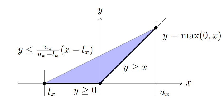
Emperically we demonstrated that regions produced by <strong>PARADE</strong> can summarize very large number of individual adversarial examples making them an useful tool to asses the robustness of neural networks. 
We hope that we piqued your interest in our work. For further details and experiments, please refer to our <a href="https://files.sri.inf.ethz.ch/website/papers/symex.pdf"><em>ICLR 2022 paper</em></a>.</p>
<h3 id="acknowledgments">Acknowledgments</h3>

<p>I would like to thank all of my collaborators for contributing to this paper. In particular, I want to thank <a href="https://ggndpsngh.github.io/"><em>Gagandeep Singh</em></a>, who supervised me on the project and is now professor at UIUC, for his help and mentorship.</p>]]></content><author><name></name></author><category term="paper" /><summary type="html"><![CDATA[We introduce the concept of provably robust adversarial examples. These are adversarial examples that are generated together with a region around them that can be proven robust to perturbations. We also show a method for generating large such regions in a scalable manner.]]></summary></entry><entry><title type="html">Multi-neuron Relaxation Guided Branch-and-bound</title><link href="https://www.sri.inf.ethz.ch/blog/mnbab" rel="alternate" type="text/html" title="Multi-neuron Relaxation Guided Branch-and-bound" /><published>2022-04-21T00:00:00+00:00</published><updated>2022-04-21T00:00:00+00:00</updated><id>https://www.sri.inf.ethz.ch/blog/mnbab</id><content type="html" xml:base="https://www.sri.inf.ethz.ch/blog/mnbab"><![CDATA[<p>This blog post explains the high-level concepts and intuitions behind our most recent neural network verifier <a href="https://files.sri.inf.ethz.ch/website/papers/ferrari2022complete.pdf">MN-BaB</a>. First, we introduce the neural network verification problem. Then, we  present the so-called Branch-and-Bound approach for solving it and outline the main ideas behind multi-neuron constraints, before combining the two in our new verifier MN-BaB. We conclude with some experimental results and insights on  why using multi-neuron constraints is key for the verification of challenging networks with high natural accuracy.</p>
<h3 id="neural-network-verification">Neural Network Verification</h3>
<p>In a nutshell, the neural network verification problem can be stated as follows:</p>

<p><em>Given a network and an input, prove that all points in a small region around that input are classified correctly, i.e., that no <a href="https://openai.com/blog/adversarial-example-research/">adversarial example</a> exists.</em></p>

<p>To formalize this a bit, we consider a network $f: \mathcal{X} \to \mathcal{Y}$, an input region $\mathcal{D} \subseteq \mathcal{X}$, and a linear property $\mathcal{P}\subseteq \mathcal{Y}$ over the output neurons $y\in\mathcal{Y}$, and we try to prove that</p>

\[f(x) \in \mathcal{P}, \forall  x \in \mathcal{D}.\]

<p>For the sake of explanation, we consider a fully connected $L$-layer network with ReLU activations but note that we can handle all common architectures. <!--as the Branch-and-Bound framework only yields complete verifiers for piecewise linear activation functions but remark that our approach applies to a wide class of activations including ReLU, Sigmoid, Tanh, MaxPool, and others.--> We denote the weights and biases of neurons in the $i$-th layer as $W^{(i)}$ and $b^{(i)}$ and define the neural network as</p>

\[f(x) := \hat{z}^{(L)}(x), \qquad \hat{z}^{(i)}(x) := W^{(i)}z^{(i-1)}(x) + b^{(i)}, \qquad z^{(i)}(x) := \max(0, \hat{z}^{(i)}(x)).\]

<p>Where $z^{(0)}(x) = x$ denotes the input, $\hat{z}$ are the pre-activation values, and $z$ the post-activation values. For readability, we omit the dependency of intermediate activations on $x$ from here on.</p>

<p>Let $\mathcal{D}$ be an $\ell_\infty$ ball around an input point $x_0$ of radius $\epsilon$: 
\(\mathcal{D}_\epsilon(x_0) = \left\{ x \in \mathcal{X} \mid \lVert x - x_0\rVert _{\infty} \leq  \epsilon \right\}.\)</p>

<p>Since we can encode any linear property over output neurons into an additional affine layer, we can simplify the general formulation of $f(x) \in \mathcal{P}$ to $f(x) &gt; {0}$. Any such property can now be verified by proving that a lower bound to the following optimization problem is greater than $0$:</p>

\[\begin{align*}
    \min_{x \in \mathcal{D}_\epsilon(x_0)} \qquad &amp;f(x) = \hat{z}^{(L)} \tag{1} \\
    s.t. \quad &amp; \hat{z}^{(i)} = W^{(i)}z^{(i-1)} + b^{(i)}\\
        &amp; z^{(i)} = \max({0}, \hat{z}^{(i)})\\
\end{align*}\]

<h3 id="background-branch-and-bound-for-neural-network-verification">Background: Branch-and-Bound for Neural Network Verification</h3>
<p>Recently, the <em>Branch-and-Bound</em> (<strong>BaB</strong>) approach, first described for this task in <a href="https://arxiv.org/pdf/1909.06588.pdf">Branch and Bound for Piecewise Linear Neural Network Verification</a>, has been popularized. At a high level, it is based on splitting the hard optimization problem of Eq. 1 into multiple easier subproblems by adding additional constraints until we can show the desired bound of $f(x) &gt; 0$ on them.</p>

<p>The high-level motivation is the following: the optimization problem in Eq. 1 would be efficiently solvable if not for the non-linearity of the ReLU function. Since a ReLU function is piecewise linear and composed of only two linear regions, we can make a case distinction between a single ReLU node being “active” (input $\geq 0$) or inactive (input $&lt; 0$) and prove the property on the resulting cases where the ReLU behaves linearly.</p>

<p>In the limit where all ReLU nodes are split, the verification problem becomes fully linear and can be solved efficiently. However, the number of subproblems to be solved in the resulting Branch-and-Bound tree is exponential in the number of ReLU neurons on which we split. Therefore, splitting all ReLU nodes is computationally intractable for all interesting verification problems. To tackle this problem, we prune this Branch-and-Bound tree using the insight that we do not have to split a subproblem further, once we find a lower bound that is $&gt;0$.</p>

<p>In pseudo-code, the Branch-and-Bound algorithm looks as follows:</p>

<figure class="highlight"><pre><code class="language-python" data-lang="python">    <span class="k">def</span> <span class="nf">verify_with_branch_and_bound</span><span class="p">(</span><span class="n">network</span><span class="p">,</span> <span class="n">input_region</span><span class="p">,</span> <span class="n">output_property</span><span class="p">)</span> <span class="o">-&gt;</span> <span class="nb">bool</span><span class="p">:</span>
      <span class="n">problem_instance</span> <span class="o">=</span> <span class="p">(</span><span class="n">input_region</span><span class="p">,</span> <span class="n">output_property</span><span class="p">)</span>

      <span class="n">global_lb</span><span class="p">,</span> <span class="n">global_ub</span> <span class="o">=</span> <span class="n">bound</span><span class="p">(</span><span class="n">network</span><span class="p">,</span> <span class="n">problem_instance</span><span class="p">)</span>
      <span class="n">unsolved_subproblems</span> <span class="o">=</span> <span class="p">[(</span><span class="n">global_lb</span><span class="p">,</span> <span class="n">problem_instance</span><span class="p">)]</span>

      <span class="k">while</span> <span class="n">global_lb</span> <span class="o">&lt;</span> <span class="mi">0</span> <span class="ow">and</span> <span class="n">global_ub</span> <span class="o">&gt;=</span> <span class="mi">0</span><span class="p">:</span>
            <span class="n">_</span><span class="p">,</span> <span class="n">current_subproblem</span> <span class="o">=</span> <span class="n">unsolved_subproblems</span><span class="p">.</span><span class="n">pop</span><span class="p">()</span>
            <span class="n">current_lb</span><span class="p">,</span> <span class="n">current_ub</span> <span class="o">=</span> <span class="n">bound</span><span class="p">(</span><span class="n">network</span><span class="p">,</span> <span class="n">current_subproblem</span><span class="p">)</span>

            <span class="k">if</span> <span class="n">current_ub</span> <span class="o">&lt;</span> <span class="mi">0</span><span class="p">:</span>
              <span class="k">return</span> <span class="bp">False</span>
            <span class="k">if</span> <span class="n">current_lb</span> <span class="o">&lt;</span> <span class="mi">0</span><span class="p">:</span>
              <span class="n">subproblem_left</span><span class="p">,</span> <span class="n">subproblem_right</span> <span class="o">=</span> <span class="n">branch</span><span class="p">(</span><span class="n">current_subproblem</span><span class="p">)</span>
              <span class="n">unsolved_subproblems</span><span class="p">.</span><span class="n">append</span><span class="p">(</span><span class="n">subproblem_left</span><span class="p">,</span> <span class="n">subproblem_right</span><span class="p">)</span>

            <span class="n">global_lb</span> <span class="o">=</span> <span class="nb">min</span><span class="p">(</span><span class="n">lb</span> <span class="k">for</span> <span class="n">lb</span><span class="p">,</span> <span class="n">_</span> <span class="ow">in</span> <span class="n">unsolved_subproblems</span><span class="p">)</span>
      <span class="k">return</span> <span class="n">global_lb</span> <span class="o">&gt;</span> <span class="mi">0</span></code></pre></figure>

<p>To define one particular verification method that follows the Branch-and-Bound approach, such as MN-BaB, all we have to do is instantiate the <strong>branch()</strong> and <strong>bound()</strong> functions.</p>

<h3 id="background-multi-neuron-constraints">Background: Multi-Neuron Constraints</h3>
<p>Before we do that, we need to understand <em>multi-neuron constraints</em> (<strong>MNCs</strong>), the second key building block of MN-BaB.</p>

<p>To bound the optimization problem in Eq. 1 efficiently, we want to replace the non-linear constraint $z = \max({0}, \hat{z})$ with its so-called linear relaxation, i.e., a set of linear constraints that is satisfied for all points satisfying the original non-linear constraint. If we consider just a single neuron, the tightest such linear relaxation is the convex hull of the function in its input-output space:</p>

<p><img src="/assets/blog/mn-bab/ConvexHull.png" alt="Convex hull ReLU abstraction" class="blogpost-img50" /></p>

<p>However, considering one neuron at a time comes with a fundamental precision limit, called the <a href="https://proceedings.neurips.cc/paper/2019/hash/246a3c5544feb054f3ea718f61adfa16-Abstract.html">(single-neuron) convex relaxation barrier</a>. It has since been <a href="https://www.sri.inf.ethz.ch/publications/singh2019krelu">shown</a>, that this limit can be overcome by considering multiple neurons jointly, thereby capturing interactions between these neurons and obtaining tighter bounds. We illustrate this improvement, showing a projection of the 4d input-output space of two neurons, below.</p>

<p><img src="/assets/blog/mn-bab/PRIMA.png" alt="PRIMA ReLU abstraction" class="blogpost-img50" /></p>

<p class="blogpost-caption"><em>The difference in tightness between the tightest single-neuron, and a multi-neuron relaxation.</em></p>

<p>We use the efficiently computable <em>multi-neuron constraints</em> from <a href="https://www.sri.inf.ethz.ch/publications/mueller2021precise">PRIMA</a>, which can be expressed as a conjunction of linear constraints over the joint input-output space.</p>

<h3 id="mn-bab-bounding">MN-BaB: Bounding</h3>

<p>The goal of the <strong>bound()</strong> method is to derive a lower bound to Eq. 1 that’s as tight as possible. The tighter it is, the earlier the Branch-and-Bound process can be terminated.</p>

<p>Following <a href="https://files.sri.inf.ethz.ch/website/papers/DeepPoly.pdf">previous</a> <a href="https://arxiv.org/abs/2103.06624">works</a>, we derive a lower bound of the network’s output as a linear function of the inputs:</p>

\[\min_{x \in \mathcal{D}} f(x) \geq \min_{x \in \mathcal{D}} a_{inp}x + c_{inp}\]

<p>There, the minimization over $x \in \mathcal{D}$ has a closed-form solution given by <a href="https://en.wikipedia.org/wiki/Hölder%27s_inequality">Hölder’s inequality</a>:</p>

\[\min_{x \in \mathcal{D}} a_{inp}x + c^{(0)} \geq a_{inp}x_0 - \lVert a_{inp} \rVert_1 \epsilon + c_{inp}\]

<p>To arrive at such a linear lower bound of the output in terms of the input, we start with the trivial lower bound $f(x) \geq z^{(L)}W + b^{(L)}$ and replace $z^{(L)}$ with symbolic, linear bounds depending only on the previous layer’s values $z^{(L-1)}$. We proceed in this manner recursively until we obtain an expression only in terms of the inputs of the network.</p>

<p>These so-called linear relaxations of the different layer types determine the precision of the obtained bounding method. While affine layers (e.g., fully connected, convolutional, avg. pooling, normalization) can be captured exactly, non-linear activation layers remain challenging and their encoding is what differentiates MN-BaB. Most importantly, MN-BaB enforces MNCs in an efficiently optimizable fashion. The full details are given in the <a href="https://files.sri.inf.ethz.ch/website/papers/ferrari2022complete.pdf">paper</a> but are rather technical and notation-heavy, so we will skip them here.</p>

<p>To derive the linear relaxations for activation layers, we need bounds on the inputs of those layers ($l_x$ and $u_x$ in the illustrations). In order to compute these lower and upper bounds on every neuron, we apply the procedure described above to every neuron in the network, starting from the first activation layer.</p>

<p>Note that if those input bounds for a ReLU node are either both negative or both positive, the corresponding activation function becomes linear and we do not have to split this node during the Branch-and-Bound process. We call such nodes “stable” and correspondingly nodes where the input bounds contain zero “unstable”.</p>

<p><img src="/assets/blog/mn-bab/stable_vs_unstable.png" alt="Alt Text" class="blogpost-img100" /></p>

<p class="blogpost-caption"><em>From Left to Right: stable inactive, stable active, unstable.</em></p>

<h3 id="mn-bab-branching">MN-BaB: Branching</h3>

<p>The <strong>branch()</strong> method takes a problem instance and splits it into two subproblems. This means deciding which unstable ReLU node to split and adding additional constraints to both resulting subproblems enforcing $\hat{z}&lt;0$ or $\hat{z}\geq0$, on the input of the split neuron.</p>

<p><img src="/assets/blog/mn-bab/split_constraints.png" alt="Alt Text" class="blogpost-img80" /></p>

<p class="blogpost-caption"><em>Illustration of the split constraints that are added to the generated subproblems.</em></p>

<p>The choice of which node to split has a significant impact on how many subproblems we have to consider during the Branch-and-Bound process until we can prove a property. Therefore, we aim to choose a neuron that minimizes the total number of problems we have to consider. To do this, we define a proxy score trying to capture the bound improvement resulting from any particular split. Note that the optimal branching decision depends on the bounding method that is used, as different bounding methods might profit differently from additional constraints resulting from the split.</p>

<p>As our bounding method relies on MNCs, we design a proxy score that is specifically tailored to them, called the <em>Active Constraint Score</em> (<strong>ACS</strong>). ACS determines the sensitivity of the final optimization objective with respect to the MNCs and then, for each node, computes the cumulative sensitivity of all constraints containing that node. We then split the node with the highest cumulative sensitivity.</p>

<p>We further propose <em>Cost Adjusted Branching</em> (<strong>CAB</strong>) to scale this branching score by the expected cost of performing a particular split. This cost can differ significantly, as only the intermediate bounds after the split layer have to be recomputed, making splits in later layers computationally cheaper.</p>

<h3 id="why-use-multi-neuron-constraints">Why use multi-neuron constraints?</h3>

<p>Using MNCs for bounding, while making the bounds more precise, is computationally costly. The intuitive argument why it still helps verification performance is that the number of subproblems solved during Branch-and-Bound grows exponentially with the depth of the subproblem tree. A more precise bounding method that can verify subproblems earlier (at a smaller depth), can therefore save us exponentially many subproblems that we do not need to solve, which more than compensates for the increased computational cost.</p>

<p>This benefit is more pronounced the larger the considered network and the more dependencies there are between neurons in the same layer. 
Most established benchmarks (e.g., from <a href="https://sites.google.com/view/vnn2021">VNNComp</a>) are based on very small networks or use training methods designed for ease of verification at the cost of natural accuracy. While this makes their certification tractable, they are less representative of networks used in practice. Therefore, we suggest focusing on larger, more challenging networks with higher natural accuracy (and more intra-layer dependencies) for the evaluation of the next generation of verifiers. There, the benefits of MNCs are particularly pronounced, leading us to believe that they represent a promising direction.</p>

<h3 id="experiments">Experiments</h3>
<p>We study the effect of MN-BaB’s components in an ablation study on the first 100 test images of the <a href="https://www.cs.toronto.edu/~kriz/cifar.html">CIFAR-10</a> dataset. We aim to prove that there is no adversarial example within an $\ell_\infty$ ball of radius $\epsilon=1/255$ and report the number of verified samples (within a timeout of 600 seconds) and the corresponding average runtime.
We consider two networks of identical architecture that only differ in the strength of their adversarial training method. ResNet6-A is weakly regularized while ResNet6-B is more strongly regularized, i.e. employs stronger adversarial training.</p>

<p><img src="/assets/blog/mn-bab/ablation_study.png" alt="Alt Text" class="blogpost-img50" /></p>

<p class="blogpost-caption"><em>Evaluating the effect of MNCs, Active Constraint Score (ACS) branching, and Cost Adjusted Branching (CAB) on MN-BaB. BaBSR is another branching method that is used as a baseline.</em></p>

<p>As expected, we see that both MNCs and Active Constraint Score branching are much more effective on the weakly regularized ResNet6-A. There, we verify 31% more samples while being around 31% faster, while on ResNet6-B we only verify 10% more samples.</p>

<p>As a more fine-grained measure of performance, we analyze the ratio of runtimes and number of subproblems required for verification on a per-property level on ResNet6-A.</p>

<p class="blogpost-wrap"><span><strong>Effectiveness of Multi-Neuron Constraints</strong>: We plot the ratio of the number of subproblems required to prove a property during Branch-and-Bound without vs. with MNCs. Using MNCs reduces the number of subproblems by two orders of magnitude on average.</span>
<img src="/assets/blog/mn-bab/ResNet6-A_n_subproblems_ratio_w_wo_MNC.png" alt="Alt Text" class="blogpost-img40" /></p>

<p class="blogpost-wrap"><span><strong>Effectiveness of Active Constraint Score Branching</strong>: We plot the ratio of the number of subproblems solved during Branch-and-Bound with BaBSR vs. ACS. Using ACS reduces the number of subproblems by an additional order of magnitude.</span>
<img src="/assets/blog/mn-bab/ResNet6-A_n_subproblems_ratio_branching.png" alt="Alt Text" class="blogpost-img40" /></p>

<p class="blogpost-wrap"><span><strong>Effectiveness of Cost Adjusted Branching</strong>: Finally, we investigate the effect of Cost Adjusted Branching on mean verification time with ACS. Using Cost Adjusted Branching further reduces the verification time by 50%. It is particularly effective in combination with the ACS scores and multi-neuron constraints, where bounding costs vary more significantly.</span>
<img src="/assets/blog/mn-bab/ResNet6-A_cab_runtime_comparison_p4c_acs.png" alt="Alt Text" class="blogpost-img40" /></p>

<h3 id="recap">Recap</h3>
<p>MN-BaB combines precise multi-neuron constraints with the Branch-and-Bound paradigm and an efficient GPU-based implementation to become a new state-of-the-art verifier, especially for less regularized networks. For a full breakdown of all technical details and detailed experimental evaluations, we recommend reading our <a href="https://www.sri.inf.ethz.ch/publications/ferrari2022complete">paper</a>. If you want to play around with MN-BaB yourself, please check out our <a href="https://github.com/eth-sri/mn-bab">code</a>.</p>]]></content><author><name></name></author><category term="paper" /><summary type="html"><![CDATA[Learn more about how multi-neuron constraints can be used in a Branch-and-Bound framework to build a state-of-the-art complete neural network verifier.]]></summary></entry></feed>